Abstract
Model code is full of names that are rarely explained: ReLU, GELU, SwiGLU, RMSNorm, AdamW. Each is a small function with a specific job, and each replaced something earlier for a reason that is easy to state. This article goes through them in plain terms — what the thing computes, what problem it fixes, and what it costs. It is deliberately the gentlest article in the series; LLM Training: The End-to-End Flow puts the same components in their systems context.
1. Why Any Activation Function at All
A neural network layer is a matrix multiply. Stack two of them and you get
which is just one matrix multiply with a different matrix. Without something nonlinear in between, a hundred layers collapse into one, and the model can only represent straight-line relationships no matter how large it is.
An activation function is that something. It is applied to every element independently, and its only requirement is to be nonlinear. Everything else — which shape, how smooth, how cheap — is engineering.
2. The Activation Lineage
2.1 Sigmoid and tanh: the ones that stopped being used
Early networks squashed every value into a fixed range: sigmoid into , tanh into .
The problem is what happens to the slope. For or so, both are almost flat, so their derivative is almost zero. During the backward pass, gradients are multiplied by that derivative at every layer, and a chain of small numbers multiplied together vanishes. Deep networks built from these trained very slowly or not at all — the vanishing-gradient problem.
2.2 ReLU: the one that fixed it
Negative inputs become zero; positive inputs pass through unchanged. Two properties made it the default for a decade. Its derivative is exactly 1 for positive inputs, so gradients pass through deep stacks without shrinking. And it is a comparison and a select — as cheap as an operation gets.
Its weakness is the flat half. A unit whose input is negative for every example in the data has zero gradient forever and never recovers, a failure mode called a dying ReLU.
2.3 GELU and SiLU: smoothing the corner
ReLU has a sharp corner at zero — the derivative jumps from 0 to 1. Two smooth alternatives dominate modern models:
where is the Gaussian cumulative distribution function and the sigmoid. Both read as “scale by how positive it probably is”. Both are near zero for very negative inputs, near for very positive inputs, and smooth in between — and both allow small negative outputs near zero, which keeps a unit from dying outright. SiLU is also called Swish.
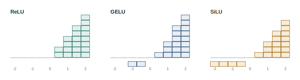
| Input | |||||
|---|---|---|---|---|---|
| ReLU | 0 | 0 | 0 | 1 | 2 |
| GELU | 0 | 0.84 | 1.95 | ||
| SiLU | 0 | 0.73 | 1.76 |
2.4 SwiGLU: adding a gate
Everything above is one function of one number. Gated activations use two:
where is elementwise multiplication. One projection produces a value, the other produces a gate that scales it. Because the two are multiplied, the layer can suppress or amplify each channel depending on the input, which a single fixed curve cannot do.
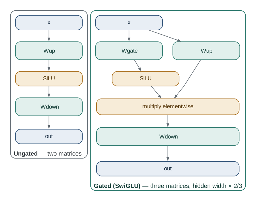
SwiGLU is what Llama, PaLM and most recent models use. The evidence for it is empirical: swapping it in improves loss at equal parameter count, and no one has a first-principles explanation. The paper that introduced the family says so outright, ending with the observation that the improvement is offered “without explanation”.
3. Normalization
Activations drifting in scale as they pass through dozens of layers makes training unstable: too large and the loss overflows, too small and gradients vanish. Normalization rescales them at every block.
LayerNorm standardizes each token’s activation vector to zero mean and unit variance, then applies a learned scale and shift:
RMSNorm drops the mean entirely and divides by the root-mean-square:
Removing the mean subtraction turns out to cost nothing in quality while saving a pass over the vector and a learned parameter, which is why current models use RMSNorm. Both are memory-bandwidth-bound: they read a vector, compute a statistic, and write a vector, with almost no arithmetic per byte.
One placement detail matters more than the choice between them. Pre-norm — normalizing the input to each sublayer, rather than its output — leaves the residual path free of any normalization, so the gradient reaches early layers unattenuated. That is what makes very deep transformers trainable without a warmup-sensitive schedule.
4. Optimizers, One Idea at a Time
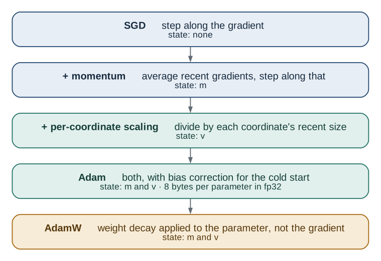
An optimizer decides what to do with the gradient once you have it. Each step below adds exactly one idea to the one before.
4.1 SGD: follow the gradient
Move each parameter a little way downhill. Simple, and it works — but every step follows the gradient of one noisy mini-batch, so the path is jittery, and one learning rate has to suit parameters whose gradients differ in magnitude by orders.
4.2 Momentum: smooth the direction
Keep a running average of recent gradients and step along that. Directions that keep reappearing accumulate; noise that flips sign cancels out. With , is roughly an average of the last ten gradients.
4.3 Per-coordinate scaling: fix the step size
Track the recent magnitude of each coordinate’s gradient and divide by it. A parameter with consistently tiny gradients gets its step scaled up; one with huge gradients gets scaled down. The learning rate stops having to be right for every parameter at once.
4.4 Adam: both at the same time
Adam keeps both averages and divides one by the other:
The hats are bias correction. Both averages start at zero, so early on they are biased toward zero and would produce tiny first steps; dividing by cancels that exactly, and the correction fades as grows.
4.5 AdamW: fix the weight decay
Weight decay keeps parameters small, which helps generalization. The old way was to add to the gradient — mathematically identical to L2 regularization for plain SGD.
With Adam it is not identical, because everything in the gradient gets divided by . A parameter with large gradients has its decay divided away to nothing; one with small gradients gets decayed hard. The regularization ends up depending on gradient history, which was never the intent.
AdamW decouples them, applying the decay to the parameter directly:
That one change is the whole difference between Adam and AdamW, and it is why every large model is trained with the latter.
| Optimizer | Extra state per parameter | Idea it adds |
|---|---|---|
| SGD | none | follow the gradient |
| SGD + momentum | smooth the direction | |
| RMSProp | per-coordinate step size | |
| Adam | , | both, with bias correction |
| AdamW | , | decoupled weight decay |
That middle column is not free. In mixed precision, and are kept in fp32 — 8 of the 16 bytes per parameter a training run has to hold, and the reason optimizer state dominates the memory budget.
5. What Gets Used Today
A current model, and why each choice is there:
| Component | Typical choice | Because |
|---|---|---|
| Activation | SwiGLU | Best measured loss at equal parameter count |
| Normalization | RMSNorm, pre-norm | Cheaper than LayerNorm; pre-norm keeps the residual path clean |
| Optimizer | AdamW | Scale-free steps, decay that behaves as intended |
| 0.9, 0.95 | Slightly faster-adapting second moment than the 0.999 default | |
| Schedule | Warmup, then cosine decay | Adam’s is unreliable in the first steps |
| Weight decay | 0.1 | Applied to weights, not to biases or normalization gains |
6. Summary
- Activations exist because stacked linear layers collapse into one. Everything after that is engineering.
- ReLU fixed vanishing gradients with a hard corner; GELU and SiLU smooth that corner and let units recover from being negative.
- SwiGLU multiplies two projections so the gate is learned and input-dependent, at the cost of a third matrix and a narrower hidden dimension.
- RMSNorm is LayerNorm without the mean subtraction, and pre-norm placement is what keeps deep stacks trainable.
- SGD → momentum → per-coordinate scaling → Adam → AdamW is one idea per step. Adam’s step is about regardless of gradient scale; AdamW’s only change is to apply weight decay to the parameter instead of the gradient.
References
- Vinod Nair and Geoffrey Hinton. Rectified Linear Units Improve Restricted Boltzmann Machines. ICML 2010.
- Dan Hendrycks and Kevin Gimpel. Gaussian Error Linear Units (GELUs). 2016.
- Prajit Ramachandran, Barret Zoph, and Quoc V. Le. Searching for Activation Functions. 2017.
- Noam Shazeer. GLU Variants Improve Transformer. 2020.
- Jimmy Lei Ba, Jamie Ryan Kiros, and Geoffrey E. Hinton. Layer Normalization. 2016.
- Biao Zhang and Rico Sennrich. Root Mean Square Layer Normalization. NeurIPS 2019.
- Ruibin Xiong et al. On Layer Normalization in the Transformer Architecture. ICML 2020.
- Diederik P. Kingma and Jimmy Ba. Adam: A Method for Stochastic Optimization. ICLR 2015.
- Ilya Loshchilov and Frank Hutter. Decoupled Weight Decay Regularization. ICLR 2019.