Intel TPP for LLM Inference: How Tensor Processing Primitives Accelerate Every Transformer Block on CPU
Published: Last Updated:
In our LLM Basics tutorial we walked through the end-to-end inference flow: tokenize → embed + position → L Transformer blocks (attention + MLP) → logits → next token. Every step boils down to matrix multiplications, element-wise ops, and softmax — “vector math end-to-end”.
This post looks at how Intel’s TPP-PyTorch-Extension maps each of those operations to highly-optimized CPU kernels, using LIBXSMM Tensor Processing Primitives (TPPs). If the first tutorial explained what is computed, this one explains how it is computed fast on an Intel Xeon.
1. What is TPP / LIBXSMM?
LIBXSMM is Intel’s open-source library of small, JIT-compiled matrix-math kernels (GEMMs, element-wise ops, transposes, VNNI/AMX micro-kernels). A Tensor Processing Primitive is a single, fused micro-kernel that operates on small tiles of a tensor — for example, a 32×32 BF16 BRGEMM (Batch-Reduce GEMM).
tpp-pytorch-extension wraps these primitives in a PyTorch C++ extension. When you call OptimizeModelForLlama(model, ...), it:
- Monkey-patches the HuggingFace model’s forward methods so that every decoder layer’s forward is routed through a C++
LlamaDecoderLayerobject. - Converts weights from plain
nn.Linearinto blocked layouts tailored for Intel VNNI / AMX instructions. - Optionally quantizes weights (MXFP4, QINT8, QINT2) at conversion time.
- Replaces the default KV cache with a custom
TppCachebacked by a C++ object, with blocked KV storage and multiple layout choices.
The result: the entire decoder stack runs in fused C++ code with OpenMP thread-level parallelism, LIBXSMM micro-kernels, and no Python overhead per layer.
2. Connecting to the LLM Basics Tutorial
Recall the stages from the LLM basics post:
| Tutorial Section | What is Computed | TPP Equivalent |
|---|---|---|
| §3 Embedding + Position | Token embedding lookup + RoPE | Precomputed RoPE table; OpenMP-parallel apply_rotary_pos_emb_llama |
| §4.2 Self-attention (Q, K, V projections) | $Q = XW_Q$, $K = XW_K$, $V = XW_V$ | Fused QKV GEMM — one, two, or three multiplications fused into a single call |
| §4.3 Multi-Head Attention | Split into heads, compute $\text{softmax}(QK^T/\sqrt{d_k})V$ | Blocked BRGEMM attention with flash-style online softmax |
| §4.4 Causal mask | Upper-triangle mask sets future scores to $-\infty$ | Inline causal masking inside the attention loop |
| §4.5–4.6 MLP / FFN | $\text{down}(\text{SiLU}(\text{gate}(x)) \odot \text{up}(x))$ | Fused GEMM + SiLU post-op, fused GEMM + element-wise multiply post-op |
| §8 KV Caching | Append K, V to a growing cache | TppCache with blocked S-dimension, multiple memory layouts |
The rest of this post dives into each of these.
3. The Fused Decoder Layer: a Bird’s-Eye View
For a Llama-style model, the C++ LlamaDecoderLayer::_forward<T>() executes the exact same mathematical flow from the tutorial, but in a single fused function (no Python loops, no autograd overhead):
flowchart TD
    IN["Input hidden_states<br/>(B × S × d)"] --> LN1["RMS Norm<br/>(input_layernorm)"]
    LN1 --> QKV["Fused QKV GEMM"]
    QKV --> Q[Q]
    QKV --> KV["K, V"]
    Q --> RQ[RoPE]
    KV --> RKV[RoPE]
    RQ --> MHA["MHA<br/>(blocked flash attention)"]
    RKV --> MHA
    MHA --> WO["Output projection W_o"]
    WO --> LN2["RMS Norm<br/>(post_attention_layernorm)"]
    LN2 --> MLP["SiLU gated MLP:<br/>gate = GEMM(x, W_gate) → SiLU<br/>up = GEMM(x, W_up) → gate * up<br/>down = GEMM(gate*up, W_down) + residual"]
    MLP --> OUT[Output hidden_states]

    LN1 -.- N1["OpenMP-parallel TPP"]
    QKV -.- N2["1 or 3 BRGEMM calls"]
    RQ  -.- N3["OpenMP collapse(3) loop"]
    MHA -.- N4["BRGEMM + online softmax"]
    WO  -.- N5["BRGEMM + residual add (fused)"]

    classDef note fill:none,stroke:none,color:#888,font-style:italic;
    class N1,N2,N3,N4,N5 note;
Every arrow above is a LIBXSMM TPP kernel call. Let’s look at each stage.
4. Intel-Specific Optimizations
4.1 Blocked Weight Layouts and VNNI
Standard PyTorch stores a linear layer’s weight as a 2-D tensor [K, C] (output features × input features). TPP converts this to a 5-D blocked layout:
where:
- $C_1 \times C_2 \times C_3 = C$ (input features), $K_1 \times K_2 = K$ (output features).
- $C_2, K_2$ are chosen to match the hardware tile size (e.g.,
bk=16, bc=64for AMX). - $C_3$ is the VNNI interleave factor (2 for BF16, 4 for INT8).
Why? Intel AMX / VNNI instructions operate on small tiles. The blocked layout keeps each tile’s data contiguous in memory, avoiding gather/scatter and maximising cache-line utilization. The conversion happens once at model-load time (FixLinear()), so inference pays zero overhead.
Toy example. Take the $4 \times 4$ query projection $W_Q$ from the LLM basics tutorial (§4.2). PyTorch stores it as a plain [4, 4] tensor. With a tile size of $2 \times 2$ and a VNNI factor of 2 (BF16), TPP reshapes it into a [2, 1, 2, 2, 2] blocked tensor. Same 16 numbers, just reordered so that each $2 \times 2$ tile sits next to each other in memory — which is how the AMX hardware wants to read them. $Q = X W_Q$ still computes the same result.
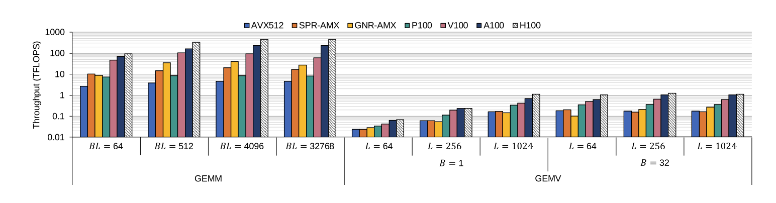
How much does this buy in practice? The figure below (from the LIA paper) shows AMX throughput on Sapphire Rapids and Granite Rapids against AVX-512 and GPUs:
4.2 Fused QKV GEMM
In the tutorial (§4.2) we wrote $Q = XW_Q$, $K = XW_K$, $V = XW_V$ as three separate multiplications. TPP offers three fusion levels controlled by the FUSED_QKV_GEMM environment variable:
| Mode | What happens |
|---|---|
FUSED_QKV_GEMM=0 | Three separate BRGEMMs (baseline). |
FUSED_QKV_GEMM=1 | Q, K, V computed in a single fused call: one loop over the input blocks writes Q, K, V outputs in-register. |
FUSED_QKV_GEMM=2 | Q, K, V plus the MLP gate projection — four outputs from one pass over the input. |
Fusion reduces the number of times the input hidden_states must be read from memory. For a d=4096 model, this cuts memory traffic by ~3× for QKV and ~4× for QKV+gate — a large win on bandwidth-limited CPUs.
4.3 Weight Remapping for First-Token (Prefill)
During the prefill pass (also called “first token”), the sequence length $S$ can be hundreds or thousands of tokens. This makes each GEMM a large matrix–matrix multiply — compute-bound rather than memory-bound.
TPP exploits this by keeping a second copy of each weight matrix in a different blocked layout optimized for large-batch GEMMs (wt_tensor_for_first_token<T>()). The decision is automatic:
bool weight_reuse = check_weight_reuse(t_HS);
if (weight_reuse && TPP_CACHE_REMAPPED_WEIGHTS) {
    t_Wq = this->t_Wq_1;  // use prefill layout
    ...
}
This burns extra memory (2× weight storage) but dramatically improves prefill throughput because the blocked layout for large-$S$ tiles better utilizes the AMX hardware.
4.4 Quantization at Load Time
FixLinear() supports transparent weight quantization:
| Format | Env / Arg | Description |
|---|---|---|
| MXFP4 | --weight-dtype mxfp4 | Microscaling 4-bit float (OCP MX standard). 4× compression. |
| QINT8 | --weight-dtype qint8 | Symmetric 8-bit integer. 2× compression. |
| QINT2 | --weight-dtype qint2 | 2-bit integer. 16× compression. |
| BFloat8 | --weight-dtype bfloat8 | 8-bit brain float. 2× compression. |
The de-quantization happens inside the BRGEMM kernel itself — the micro-kernel reads compressed weights and converts to the compute type (BF16 or FP32) on-the-fly using LIBXSMM’s data-type conversion TPPs. This means the memory bus only carries compressed data, while the ALUs still operate at full precision.
4.5 Fused Post-Ops
Every GEMM call in the decoder layer can carry a post-op — an element-wise operation fused directly after the matrix multiply, before the result is written back to memory:
| Post-Op | What it Does | Where Used |
|---|---|---|
SiluPostOp | Applies $\text{SiLU}(x) = x \cdot \sigma(x)$ | MLP gate projection |
MulPostOp(t) | Element-wise multiply with tensor t | MLP: gate * up |
AddScalePostOp(res, s) | Output = GEMM_result + s × res | Residual connections: projection + residual, down_proj + residual |
GeluPostOp | Applies GeLU activation | GPT-J / OPT MLP |
Fusing the post-op into the GEMM avoids a separate memory pass over the entire output tensor. For a 4096-wide hidden state, that saves one full read-write cycle per fused operation.
5. RoPE: Rotary Position Embedding
Recall from the basics tutorial (§3.4) that modern Llama-style models use Rotary Position Embedding (RoPE) instead of learned absolute positions. RoPE rotates pairs of dimensions in Q and K by an angle that depends on the token’s position.
In TPP, RoPE is implemented in C++ with OpenMP and operates in-place:
#pragma omp parallel for collapse(3)
for (int s = 0; s < SL; s++) {
    for (int nq = 0; nq < Nq; nq++) {
        for (int h2 = 0; h2 < H / 2; h2++) {
            auto q0 = QL[s][nq][h2];       // even dimension
            auto q1 = QL[s][nq][h2 + half]; // odd dimension
            auto cos_v = EP[s][h2];
            auto sin_v = EP[s][h2 + half];
            QL[s][nq][h2]       = q0 * cos_v - q1 * sin_v;
            QL[s][nq][h2 + half] = q1 * cos_v + q0 * sin_v;
        }
    }
}
The collapse(3) directive flattens the three loop dimensions—sequence, head, and half-dimension—into one parallel region. This gives OpenMP maximum scheduling flexibility, spreading the RoPE work evenly across all available cores. The cosine/sine tables (EP) are precomputed once at model load time by OptimizeModelForLlama() and stored as a 2-D tensor indexed by position.
6. MHA: Blocked Flash Attention with BRGEMM
The attention computation from tutorial §4.2–4.3 is:
\[\text{Attention}(Q, K, V) = \text{softmax}\!\left(\frac{QK^T}{\sqrt{d_k}}\right) V\]In raw PyTorch this would be three steps (GEMM, softmax, GEMM), each touching the full $S \times S$ attention matrix. TPP implements a blocked flash attention variant:
Block the sequence dimension into tiles of size
Sqb × Skb(query blocks × key blocks). Typical:Sqb = 64/R(where $R = N_q / N_{kv}$ for grouped-query attention),Skb = SK_BLOCK_SIZE(default 128).- For each query block (
omp parallel for collapse(3)over B, N, Sq):- For each key block in sequence:
- BRGEMM (A-GEMM): Compute a tile of $QK^T$ scores using
BrgemmTPP<T, float>. The key matrix can be in VNNI layout, and the BRGEMM handles the transposition internally. - Scale: Multiply by $1/\sqrt{d_k}$.
- Add attention mask: Add the 1-D mask (padding positions set to $-10000$).
- Causal masking: Inline: any position where
key_pos > query_posgets set to $-10^9$. - Online softmax:
VarSoftMaxFwdTPP<float, T>— maintains running max and sum across key blocks (the “flash attention” trick), avoiding ever materializing the full $S \times S$ matrix.
- BRGEMM (A-GEMM): Compute a tile of $QK^T$ scores using
- BRGEMM (C-GEMM): Multiply softmax weights × value tile.
- Softmax fixup: Rescale partial outputs from previous key blocks using the updated global max/sum (
SoftMaxFixUpTPP).
- For each key block in sequence:
- After all key blocks are processed, apply final softmax scaling (
SoftMaxFlashScaleTPP).
This approach keeps the working set small (one Sqb × Skb tile at a time) and never allocates an $S \times S$ attention matrix — critical for long-context models.
6.1 KV Cache Layouts
The KV cache from tutorial §8 is managed by TppCache. Conceptually the cache is just a big tensor of past keys and values with four dimensions:
- B — batch (which sequence)
- N — head (which attention head)
- S — sequence position (which past token)
- H — head dimension (the vector itself)
The question is only: in what order do these dimensions sit in memory? That ordering is the “layout”, and TPP supports a few because different attention steps prefer different orderings. Two extra tricks show up in the shapes below:
- The sequence dimension S is split into blocks: $S = S_1 \times S_2$, with $S_2 = 32$ tokens per block by default. A new token during decoding then only touches the last block — a cheap append.
- Some layouts pre-interleave data for VNNI instructions (the $V$ factor, 2 for BF16), so the GEMM kernels can consume the cache directly.
| Layout | Tensor Shape | When it helps |
|---|---|---|
BNSH | [S1, B, N, S2, H] | Default; natural order for most kernels. |
BNHS | [S1, B, N, H, S2] | Keys stored pre-transposed, so $QK^T$ needs no transpose at attention time. |
SBNH | [S1, S2, B, N, H] | Sequence-first; matches how tokens arrive. |
vBNSH | [S1, B, N, S2/V, H, V] | BNSH with VNNI interleaving baked in. |
vBNHS | [S1, B, N, H, S2] | BNHS with VNNI interleaving baked in. |
You don’t normally pick these by hand — the point is simply that storing the cache in the order the hardware will read it avoids transposes and data shuffling inside the attention loop. The cache also grows in pre-allocated chunks (KV_CACHE_INC_SIZE, default 128 tokens) instead of reallocating on every step.
7. OpenMP and Its Role
TPP relies on OpenMP as the sole threading model. There is no separate thread pool or custom scheduler.
7.1 Where parallelism is applied
| Operation | Parallel Strategy | Detail |
|---|---|---|
| RoPE | collapse(3) over S, N, H/2 | Fine-grained; scales to many cores |
| RMS / Layer Norm | parallel for over S | Each token normalized independently |
| Attention (MHA) | collapse(3) over B, N, Sq-blocks | Coarse; each thread owns a query tile |
| KV cache copy | collapse(3) over B, N, S-blocks | Only used when S > 1 (prefill) |
| BRGEMM kernels | Internal LIBXSMM threading | AMX tile scheduling |
7.2 Why this matters for CPU inference
On a server Xeon with 56+ cores, OpenMP’s runtime can efficiently distribute work with near-zero overhead at the parallel for sites. The collapse directive is critical: without it, the outermost loop (often batch size 1 during decoding) would serialize everything to a single core.
7.3 NUMA-aware execution
The example scripts use numactl for memory affinity:
OMP_NUM_THREADS=56 numactl -m 0 -C 0-55 python run_generation.py --use-tpp
This pins threads and memory to a single NUMA node, avoiding cross-socket traffic. For multi-socket, TPP supports tensor parallelism with distributed weight sharding (see §8).
8. Tensor Parallelism and Distributed Inference
For models that don’t fit in a single socket’s memory, TPP supports tensor parallelism across NUMA nodes or sockets:
Weight sharding (
ShardLinear()): Q, K, V, gate, up projections are sharded along the output dimension (each rank getsdim // world_sizecolumns). Down and output projections are sharded along the input dimension.SHM allreduce: After each projection or MLP output that was sharded along the input dimension, the partial results must be summed across ranks. Instead of MPI collectives, TPP uses a shared-memory allreduce (
allreduce()→shm_allreduce()), which writes directly to a shared memory buffer. This avoids the kernel-space overhead of MPI for single-node communication.Model sharding to disk: For HBM (Sapphire Rapids with on-package memory), the model can be pre-sharded and saved per-rank (
--save-sharded-model/--load-sharded-model), so each rank loads only its portion from disk directly into HBM.
9. RMS Norm with TPP
Llama uses RMS Norm (not Layer Norm). Recall that RMS Norm is:
\[\text{RMSNorm}(x) = \frac{x}{\sqrt{\frac{1}{d}\sum_{i=1}^{d} x_i^2 + \epsilon}} \cdot \gamma\]TPP implements this with two passes per token (#pragma omp parallel for over the sequence dimension):
- Compute the mean of squares.
- Scale each element by $\gamma / \text{rms}$.
Both passes use LIBXSMM reduction and element-wise TPPs, so the loop body is a single fused kernel call, not a series of PyTorch tensor operations.
10. Putting It All Together: Latency Breakdown
The command to run Llama inference with TPP:
OMP_NUM_THREADS=56 numactl -m 0 -C 0-55 \
  python run_generation.py \
    -m meta-llama/Llama-2-7b-hf \
    --device cpu --dtype bfloat16 \
    --use-tpp --weight-dtype mxfp4 \
    --max-new-tokens 128 \
    --token-latency
This:
- Loads the model from HuggingFace.
- Calls
OptimizeModelForLlama(), which:- Precomputes RoPE cosine/sine tables.
- Converts every
nn.LineartoBlockedLinearwith MXFP4 weights (4-bit). - Shards weights if running multi-process.
- Replaces all decoder layer forwards with the C++
LlamaDecoderLayer. - Installs a
TppCacheas the KV cache.
- Runs generation: first-token (prefill) uses the remapped weight layout; subsequent tokens use the standard blocked layout.
- Prints per-token latencies, broken down by first vs. subsequent tokens.
10.1 Environment variables for tuning
| Variable | Default | Description |
|---|---|---|
FUSED_QKV_GEMM | 1 | QKV fusion level (0, 1, or 2) |
TPP_CACHE_REMAPPED_WEIGHTS | 1 | Keep second weight copy for prefill |
FT_OPT_SIZE | 0 | Sequence-length threshold for using prefill layout |
KV_CACHE_INC_SIZE | 128 | Pre-allocation chunk for KV cache |
SK_BLOCK_SIZE | 128 | Key-block size in attention |
USE_FLASH | 1 | Use flash-style online softmax |
USE_SHM_ALLREDUCE | 0 | Use shared-memory allreduce instead of MPI |
11. Summary
| LLM Concept (Tutorial) | Standard PyTorch | TPP-Optimized |
|---|---|---|
| Linear layers | nn.Linear (MKL SGEMM) | BlockedLinear with VNNI/AMX BRGEMM |
| Attention | Loop or F.scaled_dot_product_attention | Blocked flash attention with TPP BRGEMM + online softmax |
| Activation (SiLU, GeLU) | Separate torch.nn.functional call | Fused post-op inside GEMM |
| Residual add | x + sublayer(x) | AddScalePostOp fused into GEMM |
| Positional encoding (RoPE) | Python loop or torch ops | In-place C++ with omp collapse(3) |
| KV cache | Python list of tensors | C++ TppCache with blocked layout + pre-allocation |
| Quantization | External library (GPTQ, bitsandbytes) | Built-in MXFP4 / QINT8 / QINT2 at weight-load time |
| Multi-socket | Separate processes + NCCL/Gloo | SHM allreduce + weight sharding, no GPU comm stack |
The key insight: by replacing Python-level tensor operations with fused, JIT-compiled LIBXSMM micro-kernels and using OpenMP for thread-level parallelism, TPP eliminates the overhead of the PyTorch dispatcher, merges memory passes (read input once → write Q, K, V, and gate), and matches the memory-access patterns to Intel VNNI/AMX hardware.
Every multiplication, normalization, and activation from the LLM basics tutorial is preserved mathematically — only the execution strategy changes.
References: