Abstract
Nearly every performance problem in training is a data-movement problem, and there are two standard answers to it. Inside a device, tiling restructures a computation so that each value loaded from slow memory is used many times before it is evicted. Between devices, collective operations move and combine data among all workers at once, at a cost that a naive point-to-point implementation cannot match. This article develops both from first principles: the arithmetic-intensity argument that says what tile size is needed, the capacity constraint that says what tile size is affordable, and then the six collectives that appear in distributed training, each with a worked four-rank example and a cost model. It builds on LLM Training: The End-to-End Flow, and it is the mechanism underneath the gradient synchronization studied in PyTorch Distributed Training Internals.
1. The Only Number That Matters
A kernel is limited either by arithmetic or by memory traffic, and which one is decided by a single ratio. The arithmetic intensity of a computation is
A device has its own ratio, the ridge point, where its peak arithmetic rate and its peak bandwidth balance:
For an H100 SXM at roughly 990 TFLOP/s of dense BF16 tensor-core throughput and 3.35 TB/s of HBM bandwidth, FLOP per byte. A kernel with cannot reach peak arithmetic no matter how well its instructions are scheduled; it is waiting on memory. The number is remarkable in itself: modern accelerators demand hundreds of operations per byte before they will run at full speed, and almost nothing achieves that naively.
Tiling exists to raise . Collectives exist because the same ratio applies across a network, where bandwidth is one to two orders of magnitude lower still.
2. Tiling
2.1 The problem, in one matrix multiply
Consider with all three matrices at bytes per element. The arithmetic is fixed at FLOPs. The traffic is not.
Computing one output element at a time reads an entire row of and an entire column of — elements — to produce a single value with FLOPs. The intensity is
one FLOP per element regardless of — and since BF16 elements are bytes, half a FLOP per byte. Every byte fetched from HBM buys half an operation, against a ridge point that demands 295, so the multiply runs some 600 times slower than the tensor cores could execute it.
Nothing is wrong with the arithmetic; the problem is that every element loaded is used exactly once.
2.2 The fix
Compute a block of instead of one element. That block needs rows of and columns of , and every one of those loaded values participates in different output elements.
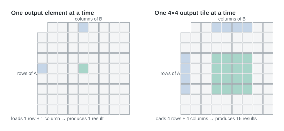
Counting the whole product takes three steps. First, is divided into
Second, producing one tile requires the strip of whose rows it spans and the strip of whose columns it spans — elements loaded, serving outputs. Third, multiply the two:
which is bytes. The same count read the other way: each element of is loaded once per block-column of , so times instead of , and likewise for . Setting returns elements, the naive schedule, as it must.
The arithmetic has not changed, so dividing the fixed FLOPs by that traffic gives
A toy example. Take in BF16 (), a single layer’s worth of matrix multiply. The arithmetic is GFLOP either way — 0.14 ms at 990 TFLOP/s. Only the traffic changes:
| Schedule | Elements read | Bytes | Time at 3.35 TB/s |
|---|---|---|---|
| One output element at a time | G | 275 GB | 82 ms |
| tiles | G | 2.1 GB | 0.64 ms |
| Lower bound: each matrix once | M | 100 MB | 0.03 ms |
The untiled schedule spends 82 ms moving data to cover 0.14 ms of arithmetic — the tensor cores are idle 99.8% of the time. Tiling at cuts that to 0.64 ms, which is a 128-fold reduction and still 4.6 times the arithmetic. That residual factor is not a rounding error; §2.3 shows it is exactly the gap between this tile’s intensity and the hardware’s ridge point.
The intensity is set by the tile size, and by nothing else. This single expression is the whole theory of tiling: make the tile as large as it can be, because intensity is linear in it.
2.3 What stops the tile from growing
Capacity. The tile must fit in the fast memory it is being reused from.
Count what has to be resident at one instant. At each step of the loop the kernel holds one chunk of and one chunk of :
Those chunks are double-buffered — while the tensor cores consume step , the copy engine is already fetching step , which is what keeps the loop from stalling on memory — so two such pairs are live at once. Multiplying by bytes per element gives the constraint:
On an H100, with up to 228 KB of shared memory per block, and in BF16 needs KB, a comfortable fit. The resulting intensity is FLOP per byte.
Note what is absent from that inequality: the output tile. Accumulators live in registers, not shared memory, which gives a second and usually tighter constraint. In fp32 they occupy bytes against a 256 KB register file per SM — 64 KB at , the whole file at .
Both numbers matter for the next question. An intensity of 64 is well below the ridge point of 295, so a tile cannot reach peak from HBM alone. Reaching 295 at would need , and such a tile needs KB of shared memory — already past the 228 KB limit — while its accumulator would need MB of registers, five times the entire file. The tile cannot grow that far on either resource.
2.4 Tiles all the way down
The consequence of the previous section is that tiling is never a single decision. Each level of the memory hierarchy gets its own tile, sized to its own capacity, nested inside the tile of the level above.
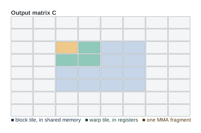
| Level | Capacity (H100) | Bandwidth | What is tiled for it |
|---|---|---|---|
| Registers | 256 KB per SM | ~20 TB/s | The MMA fragment and the accumulator |
| Shared memory | 228 KB per block | ~15 TB/s | The block tile of and , double-buffered |
| L2 | 50 MB | ~7 TB/s | The working set of a concurrent wave of blocks |
| HBM | 80 GB | 3.35 TB/s | Nothing — this is what tiling is avoiding |
Reading the table top to bottom, capacity grows by five orders of magnitude and bandwidth falls by one. Every tile boundary is a decision about which of those two facts to pay for.
2.5 The same idea outside GEMM
Tiling is not a matrix-multiply trick, and three examples from elsewhere in this series make that clear.
Attention. FlashAttention tiles the query and key dimensions and keeps the score tile on chip, never materializing the score matrix in HBM. The online-softmax recurrence exists precisely to make the tiled schedule produce the same answer as the untiled one. That is tiling with an extra requirement: the reduction over the tiled axis must be exact.
The loss. The basics article notes that logits for a large vocabulary can exceed the size of every Transformer block combined. Production trainers compute cross-entropy in chunks over the sequence — a tile over positions — so the full tensor never exists at once.
Activation checkpointing. The same trade in the time dimension: instead of holding every intermediate, hold a few and recompute the rest. Recomputation is to activation memory what tiling is to bandwidth — spend arithmetic to avoid storage.
3. Collective Operations
Tiling handles the memory hierarchy of one device. Distributed training adds a slower level below HBM — the interconnect — and the operations that cross it are collectives.
A collective is an operation that every rank in a group calls, and that completes only when all of them have. That property is what allows an implementation to schedule the transfer as a single coordinated pattern rather than as a set of independent messages.
3.1 The six that matter
The vocabulary is small. Take four ranks, each holding a vector, and the picture is complete.
| Operation | Before | After |
|---|---|---|
| Broadcast | One rank has the data | Every rank has the same copy |
| Reduce | Each rank has a vector | One rank has the elementwise sum |
| All-reduce | Each rank has a vector | Every rank has the elementwise sum |
| Reduce-scatter | Each rank has a full vector | Each rank has one distinct slice of the sum |
| All-gather | Each rank has one slice | Every rank has the whole concatenation |
| All-to-all | Each rank has one slice per destination | Each rank has one slice from every source |
Two relationships are worth committing to memory, because implementations and sharding strategies are built on them:
The first decomposition is the efficient one and the second is not, for reasons §3.4 makes precise.
3.2 A worked example
Let four ranks each hold a four-element vector:
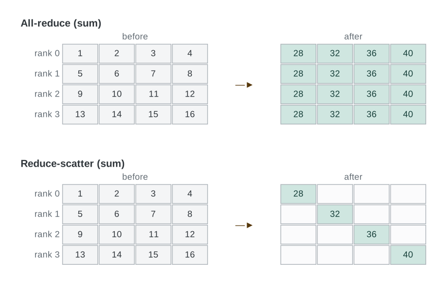
All-reduce (sum). Every rank ends with the elementwise sum of all four:
This is what DDP calls on a gradient bucket, with a division by four afterwards to make it a mean.
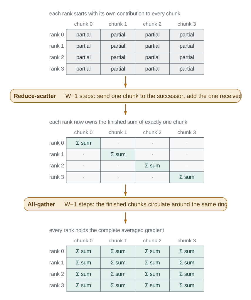
Reduce-scatter (sum). The same sums are computed, but each rank keeps only its own slice: rank 0 holds , rank 1 holds , rank 2 holds , rank 3 holds . Each rank ends with a quarter of the data. This is the first half of the ring algorithm, and it is also exactly what a sharded optimizer wants — rank only needs the gradient for the parameters it owns.
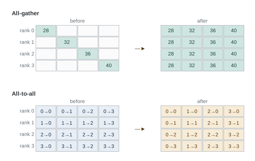
All-gather. The inverse. If rank holds the single value respectively, all-gather leaves every rank with . FSDP calls this on parameters immediately before a layer executes, and frees the result immediately after.
All-to-all. No reduction at all — a transpose across ranks. If rank holds , where is destined for rank , then afterwards rank holds . This is the collective that Mixture-of-Experts routing runs twice per layer: once to send each token to the rank owning its expert, and once to send the results back.
3.3 Reduction operators, and a warning
The combining operation is a parameter: sum, product, min, max, or average. Training uses sum almost exclusively, followed by a division.
The warning is that floating-point addition is not associative, so a collective that combined values in a different order on different ranks would return slightly different results to each of them — and in data-parallel training, where the correctness argument depends on every replica applying the identical update, that divergence compounds silently. Implementations therefore fix the reduction order for a given group and message size. It is also why changing the world size can perturb a loss curve slightly: the arithmetic is the same, the order is not.
3.4 What they cost
Model the cost of one transfer as a latency term plus a bandwidth term, for bytes on a link of bandwidth . Then for ranks and a payload of bytes per rank:
| Operation | Bytes per rank | Steps | Notes |
|---|---|---|---|
| Broadcast (tree) | Latency grows logarithmically | ||
| Reduce-scatter (ring) | Bandwidth-optimal | ||
| All-gather (ring) | Bandwidth-optimal | ||
| All-reduce (ring) | The sum of the two above | ||
| All-to-all | No reduction; pure permutation |
The naive reduce-then-broadcast decomposition is absent from that table because its cost is in bandwidth at the root: the root receives copies of the payload. The ring decomposition costs asymptotically, independent of . That difference is the entire reason collective libraries exist.
A concrete step. Take a 7B-parameter model in BF16, so the gradient is GB, on eight H100s connected by NVLink at roughly 450 GB/s per direction:
The same collective across nodes over a 400 Gb/s InfiniBand link — 50 GB/s — takes about 490 ms. Nine times the cost for the same bytes, which is why NCCL builds hierarchical rings that cross the slow level as few times as possible, and why a step whose backward pass takes 200 ms can hide the first number and cannot hide the second.
3.5 Where each one appears
| Strategy | Collective | When |
|---|---|---|
| Data parallel (DDP) | All-reduce of gradients | Once per bucket, during the backward pass |
| ZeRO / FSDP | All-gather of parameters, reduce-scatter of gradients | Per layer, forward and backward |
| Tensor parallel | All-reduce of activations | Twice per Transformer block, in both passes |
| Sequence parallel | Reduce-scatter and all-gather of activations | Replaces the tensor-parallel all-reduce |
| Pipeline parallel | Point-to-point send and receive | At each stage boundary |
| Mixture-of-Experts | All-to-all | Twice per MoE layer |
| Metrics and checkpointing | Small all-reduce, broadcast | Once per step or per checkpoint |
The rows differ in one respect that matters more than the collective they name: what the volume scales with. Data-parallel traffic scales with parameter count and is independent of batch size. Tensor-parallel and sequence-parallel traffic scales with activations, so it grows with batch and sequence length. Expert routing scales with tokens. A configuration is chosen by deciding which of those quantities the interconnect can afford to move.
4. The Same Argument, Twice
The two halves of this article are the same optimization at different scales.
Tiling raises intensity by reusing each loaded byte across more arithmetic. Ring collectives raise effective bandwidth by making every link carry useful traffic simultaneously instead of funnelling through one endpoint. Both replace a schedule whose cost grows with the size of the problem — reads per output, copies through a root — with one whose cost is bounded by the hardware’s own limits.
And both fail in the same recognizable way. A tile too large for shared memory spills; a bucket too small for the interconnect pays latency instead of bandwidth. In each case the fix comes from the same two numbers: how much fast storage there is, and how many operations each transferred byte can be made to serve.
5. Summary
- Arithmetic intensity, measured against the device’s ridge point, decides whether a kernel is limited by math or by memory. An H100 needs roughly 295 FLOP per byte.
- Tiling raises intensity linearly in the tile size, , and the tile size is capped by the capacity of the memory it is reused from. This is why tiles are nested, one per level of the hierarchy.
- The same reasoning applies outside GEMM: FlashAttention, chunked cross-entropy, and activation checkpointing are all tilings.
- Six collectives cover distributed training. All-reduce decomposes into reduce-scatter plus all-gather, and that decomposition, not reduce-plus-broadcast, is the efficient one.
- Ring collectives move bytes per rank per phase, so cost tracks payload rather than worker count — but only within a level of the interconnect hierarchy. Crossing nodes costs roughly an order of magnitude more per byte.
References
- Samuel Williams, Andrew Waterman, and David Patterson. Roofline: An Insightful Visual Performance Model for Multicore Architectures. CACM 2009.
- Pitch Patarasuk and Xin Yuan. Bandwidth Optimal All-reduce Algorithms for Clusters of Workstations. JPDC 2009.
- Rajeev Thakur, Rolf Rabenseifner, and William Gropp. Optimization of Collective Communication Operations in MPICH. IJHPCA 2005.
- Tri Dao et al. FlashAttention: Fast and Memory-Efficient Exact Attention with IO-Awareness. NeurIPS 2022.
- Vijay Thakkar et al. CUTLASS. NVIDIA, 2023.
- Samyam Rajbhandari, Jeff Rasley, Olatunji Ruwase, and Yuxiong He. ZeRO: Memory Optimizations Toward Training Trillion Parameter Models. SC 2020.