Abstract
Gradient synchronization is the one step of the training loop with no line of its own in the source: under DistributedDataParallel it is triggered from autograd hooks that fire during the backward pass. This article opens that mechanism. It contrasts DataParallel’s per-iteration replication with DDP’s persistent replicas, follows a gradient from an autograd hook through a bucket to a NCCL collective, and explains the conditions under which the communication genuinely disappears under compute. The second half is diagnostic: how to separate data, compute, communication, and overhead on a profiler timeline, and what each failure looks like. It assumes the loop and the accounting from LLM Training: The End-to-End Flow, and the collective operations and their cost models from Tiling and Collective Operations.
1. Two Ways to Use Several GPUs
Data parallelism replicates the model and splits the batch. Every replica computes a gradient from its own shard, the replicas agree on the mean, and each applies the same update. PyTorch has shipped two implementations of that idea, and the difference between them is instructive.
DataParallel (DP) is single-process and multi-threaded. One Python process drives every GPU through one thread each, and the model lives canonically on GPU 0.
DistributedDataParallel (DDP) is multi-process. Each GPU is owned by its own process with its own interpreter, its own replica, and its own optimizer. There is no privileged device.
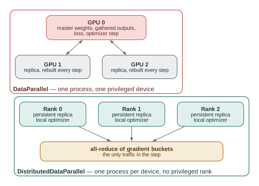
The consequences follow directly from the picture.
DataParallel | DistributedDataParallel | |
|---|---|---|
| Processes | One, with a thread per GPU | One per GPU |
| Python GIL | Shared by all device threads | Not shared |
| Model replication | Broadcast from GPU 0 every iteration | Once, at construction |
| Traffic per step | Parameters out, activations and gradients back | Gradients only |
| Loss and optimizer | On GPU 0 | On every rank, redundantly |
| Memory balance | GPU 0 holds gathered outputs | Symmetric |
| Multi-node | No | Yes |
Three of those rows are decisive. Replicating parameters every iteration moves bytes per device per step before any gradient exists — for a 7B model in bf16 that is 14 GB of broadcast per device per step, on top of the gradient traffic. Gathering every replica’s outputs to GPU 0 makes one device hold the loss inputs for the whole global batch, which is why DP runs out of memory on the first device long before the others. And one interpreter driving eight devices serializes kernel launch in Python at exactly the point where launch overhead matters most.
DP survives in the codebase as a convenience for single-machine debugging. Every production configuration uses DDP or one of its sharded descendants, and this article is about DDP.
2. What DDP Does at Construction
Wrapping a module in DDP performs three actions before training starts.
It equalizes the replicas. Rank 0 broadcasts its parameters and buffers to every other rank. This is why the correctness argument from the accounting article holds: identical initialization plus identical gradients implies identical weights, forever, with no further coordination. Loading a checkpoint on every rank independently is not equivalent unless the checkpoint is bit-identical everywhere, which is why the broadcast is unconditional.
It assigns parameters to buckets. Parameters are grouped into contiguous byte buffers of a target size, bucket_cap_mb, 25 MB by default. A bucket is the unit of communication: DDP never all-reduces a single tensor, it all-reduces a bucket.
It installs autograd hooks. Every parameter that requires a gradient receives a hook on its AccumulateGrad node. The hook does not perform communication. It copies the finished gradient into the parameter’s slice of its bucket and decrements the bucket’s pending count.
The consequence is the one that matters for performance: when the count reaches zero, that bucket is complete and its all-reduce is launched immediately — while the backward pass is still running through earlier layers.
3. The All-Reduce Itself
Every rank enters the collective with its own gradient bucket and must leave with the same average, . Tiling and Collective Operations derives what that costs: a ring implementation runs a reduce-scatter followed by an all-gather, moves bytes per rank for an -byte payload, and is therefore bounded by the payload rather than by the worker count.
What remains here is what DDP and NCCL add on top of that algorithm.
3.1 What NCCL adds
NCCL implements this and several alternatives, and chooses between them per call using payload size, worker count, and a discovered topology. Three details leak into observable performance.
The topology is hierarchical, and NCCL knows it. Intra-node NVLink or NVSwitch bandwidth is an order of magnitude above inter-node InfiniBand or Ethernet. NCCL builds rings and trees that traverse the fast links first and cross the slow ones as few times as possible, so a collective’s cost is set by the slowest level it must cross, not by an average.
Collectives consume SMs. NCCL kernels run on the GPU, using a number of channels that map to thread blocks. Communication that overlaps computation is not free: it takes streaming multiprocessors away from the compute kernels it is overlapping with. Perfectly hidden communication still slows the compute it hides behind, typically by a few percent.
Protocol selection is size-dependent. Small messages use latency-optimized protocols (LL, LL128) that trade bandwidth for fewer synchronization points; large messages use the simple protocol at full bandwidth. This is one reason very small buckets perform badly: they land in a regime where per-call overhead, not payload, sets the cost.
3.2 The volume, and why it is fixed
The payload is the gradient, so the traffic per rank per step is bytes regardless of batch size — 14 GB for a 7B model in bf16. Enlarging the micro-batch increases compute per step but not communication, which is the simplest lever for improving the compute-to-communication ratio, bounded by activation memory. Gradient accumulation is the same lever applied in time: with no_sync() on all but the last micro-step, micro-batches produce one all-reduce instead of of them.
4. Overlap, and When It Fails
The reason bucketing exists is not to reduce traffic — one all-reduce of the whole gradient would move the same bytes with fewer launches. It exists to start communicating before the backward pass finishes.
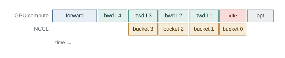
In the ideal case the only exposed communication is the last bucket, and step time is
Several things break that.
The bucket is too small. Many small collectives pay per-call overhead repeatedly and land in the latency-bound protocol regime. The symptom is a communication row full of short kernels with gaps between them.
The bucket is too large. A 500 MB bucket cannot start until the last of its gradients is ready, so a large fraction of the backward pass produces no communication at all, and the exposed tail at the end grows. The default 25 MB is a compromise between these two failures and is worth tuning for a specific model and interconnect.
Compute is faster than the link. Overlap can only hide communication under compute that exists. If , no bucketing strategy saves the step; the run is communication-bound and the fix is a larger micro-batch, gradient accumulation, or a better interconnect.
Gradients arrive in an unexpected order. Conditional execution, shared parameters, or a module whose parameters are registered in an order unrelated to execution can leave a bucket waiting on a gradient that arrives late, serializing what should have overlapped.
Unused parameters force a graph traversal. With find_unused_parameters=True, DDP walks the autograd graph on every iteration to discover which parameters produced no gradient, so their buckets can be marked ready anyway. It is correct but not free, and it is on by default in some wrappers. If the model always uses every parameter, turning it off removes a per-iteration traversal.
Two further flags matter for the same reason. gradient_as_bucket_view=True makes each parameter’s .grad a view into its bucket rather than a separate tensor, removing one copy per parameter per step and saving memory equal to the gradient set. static_graph=True tells DDP the graph does not change between iterations, which lets it retain the first iteration’s analysis instead of redoing it.
5. Where DDP Stops
DDP replicates the persistent state — all 16 bytes per parameter of it, about 112 GB for a 7B model, on every rank before a single activation is allocated, which no 80 GB device holds — the replicas fit only for models small enough that replication is affordable.
The sharded alternatives break exactly that assumption. ZeRO and its PyTorch implementation, FSDP, partition parameters, gradients, and optimizer state across the data-parallel group and reconstruct each layer’s parameters on demand. The all-reduce of DDP becomes a reduce-scatter of gradients plus an all-gather of parameters — the same two phases the ring already runs internally, but now exposed as separate operations at different points in the step.
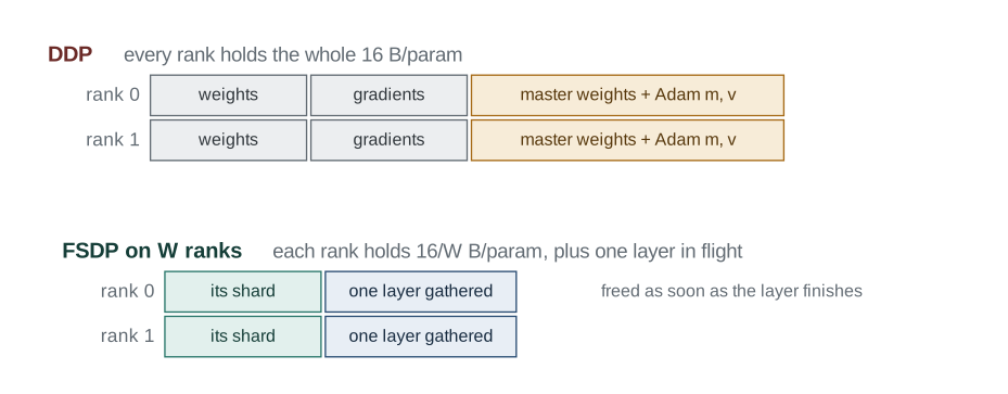
The tradeoff is traffic for memory. FSDP moves parameters as well as gradients, so its per-step volume is higher; what it buys is that per-rank persistent memory falls by a factor of the world size. The diagnostic vocabulary is unchanged: the question is still whether the collectives overlap the compute.
6. Telling the Four Buckets Apart
The accounting article identified four consumers of wall-clock time: data, compute, communication, and overhead. Attributing a slow run to one of them is a measurement problem, and the first rule is negative.
Do not diagnose from nvidia-smi. As the accounting article explains, its utilization figure counts any resident kernel, so a dataloader-starved loop and a saturating GEMM both read 100%.
What separates them is a timeline: what ran, on which stream, when, and what the CPU was doing meanwhile.
6.1 The signatures
| Bucket | On the timeline | Confirming test |
|---|---|---|
| Data | A gap before the first kernel of each step; CPU busy in dataloader workers or blocked on I/O | Replace the loader with a cached synthetic batch; if step time collapses, it was data |
| Compute | Kernels back to back, high occupancy, no gaps | Step time scales with , , and as the FLOP model predicts |
| Communication | ncclKernel entries that are not concurrent with compute kernels | Step time flat in but growing with world size; single-rank step time much lower |
| Overhead | Many short kernels separated by launch gaps; CPU-side time exceeds GPU time | The gaps persist when the batch size grows |
The word doing the work in row three is exposed. A profile full of NCCL kernels is not evidence of a communication problem; NCCL kernels running while the compute stream is idle is.
6.2 PyTorch Profiler
torch.profiler instruments both sides and exports a Chrome trace:
from torch.profiler import profile, schedule, ProfilerActivity

with profile(
    activities=[ProfilerActivity.CPU, ProfilerActivity.CUDA],
    schedule=schedule(wait=1, warmup=2, active=3),   # skip DDP's first-step rebuild
    on_trace_ready=torch.profiler.tensorboard_trace_handler("./trace"),
    record_shapes=True,
    with_stack=True,
) as prof:
    for step, batch in enumerate(loader):
        train_step(batch)
        prof.step()
The wait/warmup phases are not decoration. The first iteration includes DDP’s bucket rebuild, cuDNN and cuBLAS autotuning, and allocator growth; profiling it measures startup rather than steady state.
Read the resulting trace in this order: find the step boundary, measure the gap before the first kernel (data), check whether NCCL kernels overlap compute kernels (communication), then look at the density of the compute stream (overhead). Annotate regions with torch.profiler.record_function("name") to make phases findable.
6.3 Nsight Systems
The PyTorch profiler sees what PyTorch does. Nsight Systems sees the whole process — CUDA runtime calls, memory transfers, other libraries, kernel launch latency, and the CPU threads driving them:
nsys profile -t cuda,nvtx,osrt --capture-range=cudaProfilerApi \
    -o step_profile python train.py
Use it when the PyTorch trace shows a gap it cannot explain: host-side synchronization, an unpinned host buffer forcing a staged copy, a page-fault storm, or launch latency from a CPU that cannot keep ahead of the GPU. Wrapping phases in NVTX ranges (torch.cuda.nvtx.range_push) makes the timeline navigable.
6.4 The usual data-pipeline findings
The data bucket has a small set of recurring causes, and they are cheap to check:
num_workers=0, so decoding happens in the training process, serialized against launch.pin_memory=False, forcing a staging copy on every host-to-device transfer instead of a direct DMA from pinned memory.persistent_workers=False, so workers are torn down and respawned every epoch.- A
prefetch_factortoo small to cover a step, so the loader is always one batch behind. - Per-sample work that belongs offline — tokenization above all, which should have produced a token stream once, not once per epoch.
The concluding rule from the accounting article applies here too: fix the bucket the timeline names, not the one that is easiest to change.
7. Summary
DataParallelreplicates the model per iteration and centralizes the loss on one device; DDP replicates once and keeps every rank symmetric. Use DDP.- DDP’s hooks copy each finished gradient into a bucket; a bucket’s all-reduce launches as soon as its last gradient arrives, which is why communication overlaps the backward pass without appearing in the training loop.
- Ring all-reduce moves bytes per rank, so cost tracks model size, not cluster size, until latency terms take over.
- Overlap fails for identifiable reasons — buckets too small or too large, compute too fast for the link, gradients arriving out of order — and each has a signature on a timeline.
- Diagnose from a timeline, never from a utilization percentage, and always after the first iteration.
References
- Shen Li et al. PyTorch Distributed: Experiences on Accelerating Data Parallel Training. VLDB 2020.
- Pitch Patarasuk and Xin Yuan. Bandwidth Optimal All-reduce Algorithms for Clusters of Workstations. JPDC 2009.
- Alexander Sergeev and Mike Del Balso. Horovod: Fast and Easy Distributed Deep Learning in TensorFlow. 2018.
- Samyam Rajbhandari, Jeff Rasley, Olatunji Ruwase, and Yuxiong He. ZeRO: Memory Optimizations Toward Training Trillion Parameter Models. SC 2020.
- Yanli Zhao et al. PyTorch FSDP: Experiences on Scaling Fully Sharded Data Parallel. VLDB 2023.
- NVIDIA. NCCL Developer Guide.