Neural Network Quantization

Abstract

Quantization replaces a network’s floating-point tensors with low-precision integers plus a small number of scale factors. The arithmetic is elementary; what makes it a systems topic is that the error it introduces is not spread evenly across a transformer. A handful of activation channels carry magnitudes two orders larger than the rest, and a single per-tensor scale sized to accommodate them leaves the remaining channels with almost no resolution. This article develops the quantization map and its error, distinguishes the granularities at which scales can be attached, contrasts post-training quantization with quantization-aware training, and works through why attention and normalization are disproportionately sensitive to INT8 — then covers the methods that repair the damage. It closes on what quantization actually makes faster, which is not the same question as what it makes smaller.

1. Why Quantize

The final stage of the training lifecycle in LLM Training: The End-to-End Flow is compression, and quantization is its dominant form. Three distinct benefits are usually conflated:

Benefit	Mechanism	Where it applies
Capacity	Fewer bytes per weight	Fitting a model on a given device
Bandwidth	Fewer bytes moved per token	Decode, which is memory-bound
Throughput	Higher integer arithmetic rate	Prefill and training, which are compute-bound

They come apart in practice. Autoregressive decode reads the entire weight matrix to produce one token, so its cost is bytes moved, and halving the weight width nearly halves the time regardless of what the arithmetic runs in. Prefill multiplies large matrices and is limited by the arithmetic rate, so it only speeds up if the multiply itself happens in low precision. This distinction decides which quantization scheme is worth implementing, and §7 returns to it.

2. The Affine Map

Quantization approximates a real tensor by an integer grid. With scale $s > 0$ and integer zero-point $z$ , the forward map and its inverse are

q = \operatorname{clamp}\!\left(\left\lceil \frac{x}{s} \right\rfloor + z,\; q_{\min},\, q_{\max}\right), \qquad \hat{x} = s\,(q - z),

where $\lceil\cdot\rfloor$ is round-to-nearest and $[q_{\min}, q_{\max}]$ is the integer range — $[-128, 127]$ for signed INT8, $[0, 255]$ for unsigned.

Two variants matter. Symmetric quantization fixes $z = 0$ and sets $s = \max|x| / q_{\max}$ ; the grid is centered on zero, and the dequantization multiply is a single scalar. Asymmetric quantization allows $z \neq 0$ , so the grid can cover a range that is not centered — necessary for tensors like post-ReLU or post-softmax activations that are one-sided. Symmetric is cheaper: a nonzero zero-point introduces cross terms in the matrix product that must be computed and subtracted.

DetourWhere the error comes from

Two independent errors are in play, and they trade against each other through one knob: the clipping range.

Rounding error is bounded by half a step, $|x - \hat{x}| \le s/2$ . Treated as uniform noise it has variance $s^2/12$ , so it falls quadratically as the range narrows.

Clipping error is unbounded: any value outside $[q_{\min}, q_{\max}]$ after scaling is truncated to the endpoint, and the error is the full excess.

A wide range eliminates clipping and coarsens every step; a narrow range gives fine steps and clips the tails. Calibration is the search for the point between them, which is why min–max is rarely the best choice: a single outlier sample sets the range for the entire tensor and degrades resolution everywhere else.

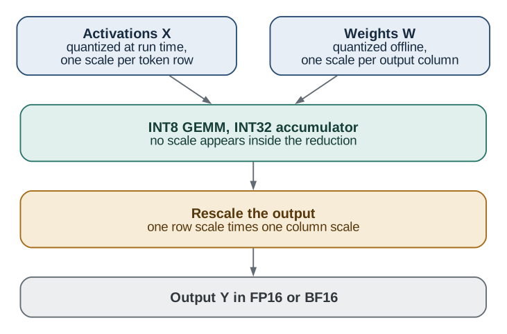
For a matrix product the scales factor out of the reduction. With symmetric per-tensor quantization of both operands,

y_{ij} = \sum_k x_{ik} w_{kj} \approx s_x s_w \sum_k q^{x}_{ik} q^{w}_{kj},

so the inner loop is an integer multiply-accumulate into an INT32 accumulator, and the two scales apply once to the result. This is the whole reason integer quantization is fast: the expensive part of the computation never touches a floating-point scale.

Quantized activations and weights entering an INT8 matrix multiply with an INT32 accumulator, whose output is rescaled by a row scale and a column scale and returned in floating point. — **Figure 1.** Where the scales are and are not. The reduction (green) is pure integer arithmetic; every floating-point scale is applied once per output element afterwards (amber). Any scheme that puts a scale inside the green box gives up this structure, which is the constraint behind everything in the next section.

3. Granularity: Where the Scales Live

A scale can be shared by an entire tensor, by a row or column, or by a small group of elements. The choice is a tradeoff between accuracy and where the scale lands in the arithmetic.

Granularity	One scale per	Cost in the GEMM
Per-tensor	Whole tensor	Free — one scalar on the output
Per-channel (weights, output dim)	Output column	Free — a vector on the output columns
Per-token (activations, row)	Input row	Free — a vector on the output rows
Per-group	Block of $k$ elements along the reduction	Not free — the reduction must be split

The pattern in the third column is the important one. A scale is free when it is constant along the reduction axis, because it can be pulled out of the sum and applied afterwards. Weight scales along the output dimension and activation scales along the token dimension both satisfy this. A scale that varies along the reduction — per-input-channel activation scaling, for instance — sits inside the sum and cannot be factored out, which is why group-wise quantization requires kernels that break the reduction into segments and rescale between them.

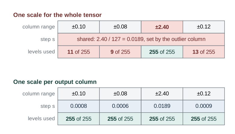
A weight matrix quantized with one shared scale, where an outlier column forces every other column onto a coarse grid, beside the same matrix with one scale per column. — **Figure 2.** Why per-channel scaling exists. With one scale for the whole tensor (top), the widest column sets the step size and the three narrow columns are left with barely a dozen of the 255 available levels each. Per-column scales (bottom) give every column the full grid, and cost nothing in the GEMM because the scale multiplies an output column.

The practical default for INT8 inference is per-channel symmetric weights and per-token activations. Weight-only schemes at 4 bits go further and use per-group scales, typically one per 64 or 128 elements along the reduction, accepting the kernel complexity because the accuracy at 4 bits demands it.

4. Post-Training Quantization and Quantization-Aware Training

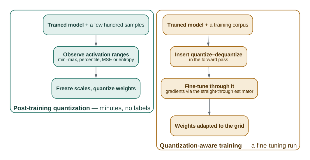
Post-training quantization (PTQ) takes a trained model and a few hundred representative samples, records the activation ranges those samples produce, chooses a clipping range per tensor, and emits the quantized weights. It costs minutes and needs no labels, no gradients, and no training infrastructure.

The choice of clipping range is the entire method:

Min–max takes the observed extremes. Simple, and maximally sensitive to a single outlier.
Percentile clips at, say, the 99.9th percentile of observed magnitudes, trading a little clipping error for a much finer step.
MSE searches for the range minimizing $\mathbb{E}\|x - \hat{x}\|^2$ over the calibration set.
Entropy (KL divergence) picks the range whose quantized distribution best preserves the information in the original, the classic TensorRT calibrator.

Quantization-aware training (QAT) instead inserts the quantize–dequantize pair into the forward pass and fine-tunes through it, so the weights adapt to the grid they will be evaluated on. The obstacle is that $\lceil\cdot\rfloor$ has zero gradient almost everywhere, which would stop backpropagation dead. The straight-through estimator resolves this by defining the backward pass of the rounding operation to be the identity within the clipping range and zero outside it:

\frac{\partial \hat{x}}{\partial x} \approx \begin{cases} 1, & q_{\min} \le x/s + z \le q_{\max},\\ 0, & \text{otherwise.} \end{cases}

Two pipelines side by side: post-training quantization observes ranges on a calibration set and freezes scales, while quantization-aware training inserts fake quantization into the forward pass and fine-tunes through it. — **Figure 3.** The two pipelines. PTQ only ever runs the model forward, which is why it needs no labels and finishes in minutes. QAT puts the quantizer inside the training loop, so the weights move to places the grid represents well — and pays a fine-tuning run for it.

The gradient that reaches the weights is therefore the gradient of the dequantized value, which is what makes the weights move somewhere the grid represents well. Later work makes the step size itself a learned parameter rather than a calibration constant.

	PTQ	QAT
Data needed	Hundreds of unlabeled samples	A fine-tuning corpus
Cost	Minutes	A training run
Typical floor	INT8, and INT4 for weights only	INT4 activations and below
When it is the right call	Almost always, first	When PTQ has been tried and the accuracy gap is unacceptable

For LLMs the balance tilts hard toward PTQ, simply because a QAT run on a model of that size costs what pretraining costs. Most of the methods in §6 are PTQ methods for exactly this reason.

5. Why Transformers Are Hard

The theory above is precision-agnostic. What makes a transformer harder to quantize than a convolutional network is the distribution of its activations.

Activation outliers are systematic, not random. Beyond roughly 6–7B parameters, transformers develop a small number of hidden dimensions — often a fraction of a percent of the total — whose magnitudes are 20 to 100 times the rest, and the same dimensions are outliers across essentially all tokens. They are not noise; the network uses them, and clipping them destroys accuracy. But keeping them inside a per-tensor range means the step $s$ is set by an outlier, and the ordinary channels are left occupying a handful of levels out of 256.

The bad axis is the expensive one. These outliers live along the hidden dimension, which is the reduction axis of the next matrix multiply. By the rule in §3, a scale along that axis cannot be factored out of the sum. The natural fix is exactly the one the hardware makes inconvenient.

Softmax outputs are one-sided and extremely skewed. Attention probabilities lie in $[0,1]$ , with most mass near zero and a few entries near one. A symmetric grid wastes half its levels on negative numbers that cannot occur, and a uniform grid spends its resolution where the values are not.

Normalization changes the scale mid-network. RMSNorm divides by a per-token statistic, so the tensor’s dynamic range depends on the token. A per-tensor activation scale calibrated on average tokens is wrong for atypical ones, which is the direct argument for per-token activation scales.

The residual stream grows with depth. Each block adds to the residual, so activation magnitudes at layer 40 are substantially larger than at layer 2. A single scale for a tensor that appears at every depth is a poor fit at both ends.

The KV cache has its own asymmetry. Keys exhibit channel-wise outliers, while values are comparatively uniform — so quantizing the cache well means quantizing keys per channel and values per token, with different kernels for each.

6. Recovering the Accuracy

The methods in production use are responses to the specific pathologies above rather than general-purpose improvements.

Mixed-precision decomposition (LLM.int8()) keeps the outlier dimensions in FP16 and quantizes everything else to INT8, splitting the matrix multiply into a small high-precision part and a large integer part. It preserves accuracy exactly where it matters, at the cost of a decomposed kernel and irregular memory access.

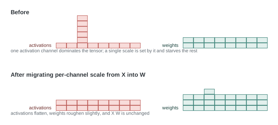
Difficulty migration (SmoothQuant) observes that a per-channel scale factor can be moved from the activations, where it is expensive, into the weights, where it is free. Choosing a per-channel factor $s_j$ and rewriting

Y = (X \operatorname{diag}(s)^{-1})\,(\operatorname{diag}(s)\,W)

leaves the product unchanged while flattening the activation outliers and mildly roughening the weights, which are easy to quantize to begin with. The exponent balancing the two, $s_j = \max|X_j|^{\alpha} / \max|W_j|^{1-\alpha}$ , is the method’s one hyperparameter.

Per-channel range charts before and after migration: one activation channel towers over the others while weights are uniform, then activations are level and weights are slightly raised in the migrated channel. — **Figure 4.** Migration in one picture. Before, a single activation channel is several times the rest, so any per-tensor activation scale is set by it. Dividing the activations by a per-channel factor and multiplying the corresponding weight rows by the same factor leaves the product identical, flattens the activation profile, and costs only a mild roughening of a tensor that was easy to quantize to begin with.

The result is that plain W8A8 becomes viable on models where it previously was not.

Error-compensating weight quantization (GPTQ) quantizes a layer’s weights one column at a time and, after each column, updates the remaining unquantized columns to compensate for the error just introduced, using second-order information from a calibration set. It is what makes 4-bit and 3-bit weight-only quantization hold up.

Salience-aware scaling (AWQ) starts from the observation that weight channels are not equally important: importance is determined by the magnitude of the activations they multiply. Protecting the salient one percent by scaling them up before quantization recovers most of the loss without backpropagation or reconstruction.

Leaving parts alone. The cheapest technique remains keeping the embedding, the output projection, and the normalization layers in higher precision. They are a small fraction of the parameters and a large fraction of the sensitivity.

7. What Actually Gets Faster

A quantized model is smaller by construction. Whether it is faster depends on which regime it runs in.

Decode is bandwidth-bound. Generating one token reads every weight once, and the arithmetic intensity is close to one operation per byte — three hundred times below the ridge point of the hardware it runs on. Weight-only quantization — INT4 weights with FP16 activations — cuts the bytes read by nearly four and speeds decode up accordingly, even though the multiply still happens in floating point after an on-the-fly dequantization. The kernel requirement is that dequantization be fused into the GEMV so the FP16 weights never round-trip to memory.

Prefill is compute-bound. Long-prompt processing multiplies large matrices, so time is set by the arithmetic rate. Weight-only quantization does nothing here — it may even lose, since dequantization is extra work. The gain requires quantizing activations as well, so the multiply itself runs on integer or FP8 tensor cores.

FP8 is the other option on recent hardware. The E4M3 and E5M2 formats keep an exponent field, so they absorb dynamic range that INT8 has to handle with scale factors, which makes them markedly more tolerant of the outliers in §5. Where the hardware supports it, FP8 with per-tensor scaling is often simpler and closer to lossless than INT8 with elaborate per-channel machinery.

Scheme	Weights	Activations	Helps decode	Helps prefill
W8A8 INT8	INT8	INT8	Yes	Yes
W4A16 weight-only	INT4	FP16	Strongly	No
FP8 (E4M3)	FP8	FP8	Yes	Yes
KV-cache only	Unchanged	Unchanged, cache in INT8/INT4	Yes, at long context	No

The last row is worth separating out. At long context the KV cache, not the weights, dominates both memory and the bandwidth of each decode step, so quantizing the cache alone can be the single largest win — and it is orthogonal to whatever is done to the weights.

8. Summary

Quantization is an affine map to an integer grid; its error is a tradeoff between rounding, which shrinks with the range, and clipping, which grows with it.
A scale is free exactly when it is constant along the reduction axis. Per-channel weight scales and per-token activation scales are free; per-input-channel activation scales are not.
PTQ is cheap and should be tried first; QAT buys the lower bit widths at the cost of a training run, which for an LLM is rarely justified.
Transformers are hard to quantize because of systematic activation outliers along the reduction axis, one-sided softmax outputs, per-token normalization statistics, and a residual stream that grows with depth.
The production methods each answer one of those: decomposition isolates outliers, SmoothQuant migrates them into the weights, GPTQ compensates the error it introduces, AWQ protects the salient channels.
Smaller and faster are different claims. Decode responds to fewer weight bytes; prefill responds only to lower-precision arithmetic.

References

Benoit Jacob et al. Quantization and Training of Neural Networks for Efficient Integer-Arithmetic-Only Inference. CVPR 2018.
Markus Nagel et al. A White Paper on Neural Network Quantization. 2021.
Yoshua Bengio, Nicholas Léonard, and Aaron Courville. Estimating or Propagating Gradients Through Stochastic Neurons for Conditional Computation. 2013.
Steven K. Esser et al. Learned Step Size Quantization. ICLR 2020.
Tim Dettmers et al. LLM.int8(): 8-bit Matrix Multiplication for Transformers at Scale. NeurIPS 2022.
Guangxuan Xiao et al. SmoothQuant: Accurate and Efficient Post-Training Quantization for Large Language Models. ICML 2023.
Elias Frantar et al. GPTQ: Accurate Post-Training Quantization for Generative Pre-trained Transformers. ICLR 2023.
Ji Lin et al. AWQ: Activation-aware Weight Quantization for LLM Compression and Acceleration. MLSys 2024.
Paulius Micikevicius et al. FP8 Formats for Deep Learning. 2022.

Abstract#

1. Why Quantize#

2. The Affine Map#

3. Granularity: Where the Scales Live#

4. Post-Training Quantization and Quantization-Aware Training#

5. Why Transformers Are Hard#

6. Recovering the Accuracy#

7. What Actually Gets Faster#

8. Summary#

References#