Abstract
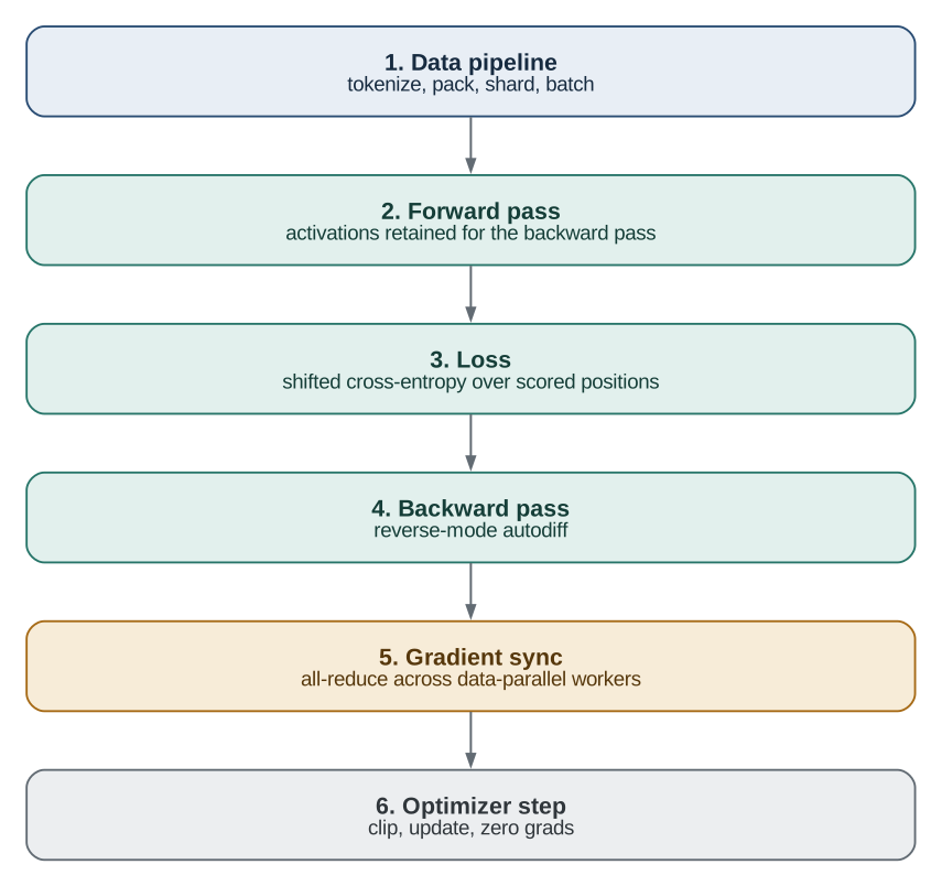
Large language model training is a loop with six recognizable steps:
- Data pipeline — fetch a batch.
- Forward pass — compute activations and retain them.
- Loss — score the predictions against the targets.
- Backward pass — propagate gradients back through the network.
- Gradient sync — all-reduce gradients across workers.
- Optimizer step — apply the update and zero the gradients.
Each step has a distinct cost profile, and each fails in a distinct way at scale. This article walks the loop end to end, establishes the memory and arithmetic accounting that decides what fits on a GPU, and identifies where wall-clock time actually goes. It is the shared vocabulary for the rest of this series, which takes individual steps apart on real hardware.
1. Training Is Not Inference Run Backwards
Both training and inference evaluate the same Transformer blocks, so the per-layer math developed in LLM Inference Introduction carries over unchanged. The systems behavior does not.
| Property | Inference | Training |
|---|---|---|
| Passes per batch | Forward only | Forward, then backward |
| Sequence handling | Prefill, then one token per decode step | Whole sequence in a single pass |
| Intermediate reuse | KV cache across decode steps | Activations retained for the backward pass |
| Resident state | Weights and KV cache | Weights, gradients, optimizer state, activations |
| Batch composition | Requests arriving over time | Fixed-shape token batches from a static corpus |
| Dominant metric | Time to first token, tokens/s per request | Tokens/s, model FLOPs utilization, loss curve |
Two consequences matter for everything that follows. First, training has no KV cache: every position in the sequence is a training example, all positions are computed at once, and there is nothing to carry forward. Second, the forward pass cannot discard its intermediates. The backward pass needs them, so activation memory becomes a first-class capacity constraint that inference simply does not have.
A single linear layer shows why. Both settings evaluate , but inference is finished with the moment exists — nothing downstream reads it. Training must eventually compute the parameter gradient
and only becomes available after the remaining layers and the loss have run. The gradient formula is a function of the layer’s input, so must stay resident from the moment it is produced until the backward pass walks back to this layer. The same holds wherever the local Jacobian is data-dependent: an activation function needs its input, softmax its output, normalization its per-row statistics.
The consequence is a factor of in the memory bound. Inference frees layer ’s buffers as soon as layer has consumed them, so its activation working set is one layer deep; training holds every layer at once:
where is bytes per element and counts the retained tensors of shape per layer, typically on the order of ten. For , , , , and bf16, one such tensor is 268 MB: about 2.7 GB of live intermediates per layer, and roughly 86 GB across the stack — more than an H100 holds, before any weights or optimizer state. The same model decoding one token at a time () keeps 32 KB per tensor.
That gap is the reason activation checkpointing is standard practice rather than an optimization. Section 3.2 revisits the bound with attention’s quadratic term.
2. The Training Lifecycle
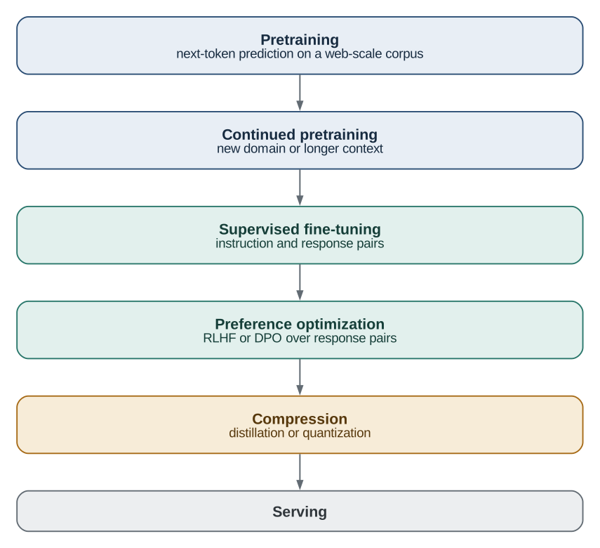
“Training an LLM” refers to a pipeline of stages with different objectives and wildly different compute budgets.
| Stage | Objective | Data scale | Share of total compute |
|---|---|---|---|
| Pretraining | Next-token cross-entropy on web text | – tokens | Dominant |
| Continued pretraining | Same objective, new distribution or longer context | – tokens | Small |
| Supervised fine-tuning | Cross-entropy on the response only | – tokens | Very small |
| Preference optimization | Rank preferred responses above rejected ones | – comparisons | Very small |
| Compression | Match a teacher, or recover accuracy at lower precision | Task-dependent | Very small |
The stages differ in objective and data, but from the first stage to the last they run the same iteration structure. The rest of this article describes that iteration.
3. One Iteration, Six Steps
3.1 Data Pipeline
The corpus is tokenized once, offline, into a flat stream of token IDs. Training does not consume variable-length documents; it consumes fixed-length windows, because fixed shapes keep GPU kernels and collective operations uniform across steps. Documents are therefore packed: concatenated end to end with a separator and cut into windows of exactly tokens.
A single training batch is a tensor of token IDs
where is the micro-batch size on one device and is the sequence length. The batch that the optimizer actually sees is larger:
where is the number of gradient-accumulation micro-steps and is the number of data-parallel workers. This identity is the main knob in distributed training: it lets a target global batch size be held fixed while is reduced to fit memory, or is increased to add hardware.
Each worker must read a disjoint shard of the data. Two workers that draw the same samples do redundant work and quietly change the effective batch composition. The shard assignment must also be deterministic in the epoch and seed, so that a job resumed from a checkpoint does not replay data it has already consumed.
This step runs on CPU while the GPU is busy with the previous batch — which is exactly why it is the most common source of GPU idle time, and why the article on distributed training spends a section on diagnosing it.
3.2 Forward Pass
The forward pass is the inference computation, applied to the whole window at once. Token IDs become embeddings, Transformer blocks apply causal self-attention and a position-wise feed-forward network, and a final projection produces logits over the vocabulary:
Two differences from the inference forward pass are important.
Every position is supervised. Inference cares only about the last position’s logits, since that is what produces the next token. Training computes a prediction at every one of the positions and scores all of them. This is what makes next-token prediction so sample-efficient: a single sequence of length yields supervised examples, and the causal mask is what makes it valid to score them in parallel without leakage. Training on the ground-truth prefix rather than the model’s own past predictions is called teacher forcing.
Intermediates are retained. Each operation saves whatever its gradient formula will need — layer inputs, normalization statistics, attention probabilities, activation-function inputs. These saved tensors form the autograd graph, and their total size scales as
with an additional term per layer for any attention implementation that materializes the score matrix. Avoiding that quadratic term is precisely what FlashAttention does, which is why it is a memory technique before it is a speed technique.
The logits tensor deserves separate attention. At , a batch of , in bf16 needs roughly 8 GB for the logits alone, and the cross-entropy computation typically needs another copy. On large-vocabulary models this single tensor can exceed the memory of every Transformer block combined, which is why production trainers compute the loss in chunks over the sequence.
3.3 Loss
The objective is the mean negative log-likelihood of the next token:
where is the softmax over the logits at position and is the set of scored positions.
Two implementation details cause more silent bugs than any other part of the loop.
The shift. The prediction at position is compared against the token at position . In code this is an off-by-one alignment between logits and labels, and getting it wrong produces a model that trains to a plausible-looking loss while learning to copy its input.
The mask . Padding tokens must be excluded. In supervised fine-tuning, prompt tokens are usually excluded too, so that the model is scored only on the response it is supposed to produce. Whether the mean is taken over tokens in the micro-batch or over tokens in the global batch also matters: with variable numbers of scored tokens per micro-batch, averaging per micro-batch and then averaging across workers silently weights workers unequally.
Loss is reported in nats per token. Its exponential, , is perplexity — the effective number of tokens the model is choosing between.
3.4 Backward Pass
The backward pass computes by reverse-mode automatic differentiation. Starting from at the output, it walks the autograd graph in reverse, and at each node applies that operation’s vector-Jacobian product to convert the gradient with respect to the node’s output into gradients with respect to its inputs and parameters.
A single linear layer shows where the cost comes from. The forward pass of is one matrix multiplication. Given , the backward pass computes two:
One produces the parameter gradient; the other propagates the signal to the previous layer. This 2:1 ratio is why the backward pass costs roughly twice the forward pass, and why the standard estimate for a full training step is about three times the forward cost.
The backward pass also frees memory as it goes: once a saved activation has been consumed, it can be released. Peak activation memory therefore occurs at the transition from forward to backward, not at the end of either.
Activation checkpointing trades this memory for compute. Selected activations are dropped during the forward pass and recomputed on demand during the backward pass. The saving is large — for uniform per-layer checkpointing, activation memory drops from to roughly under the classic scheme — at the price of one extra forward pass, raising step cost from about to about the forward pass.
3.5 Gradient Synchronization
On a single device this step does not exist. With data-parallel workers, each has computed a gradient from its own shard, and the workers must agree on their mean before any of them updates:
This is an all-reduce: every worker contributes a value and every worker receives the same result. The volume moved is proportional to the model’s parameter count, on every step, regardless of batch size — a 7B model in bf16 moves roughly 14 GB of gradient per step per worker, which is why interconnect bandwidth, not FLOPs, sets the ceiling on many training clusters.
Because the resulting gradient is identical on every worker and every worker started from identical weights, the optimizer step keeps the replicas bit-consistent without any further communication. That invariant — identical initialization plus identical gradients implies identical weights — is the entire correctness argument for data-parallel training.
Gradient accumulation interacts directly with this step. During the first micro-steps, gradients accumulate locally and synchronization is skipped; only the final micro-step synchronizes. Skipping it is not an optimization detail but a requirement: synchronizing every micro-step multiplies communication volume by for no change in result.
What an all-reduce costs and how a ring implementation achieves it is the subject of the next article; how gradients are grouped into buckets and overlapped with the backward pass is the subject of the one after that.
3.6 Optimizer Step
Before the update, gradients are usually clipped by global norm:
with computed across all parameters jointly. This bounds the damage from a rare bad batch, which in a run of hundreds of thousands of steps is a near-certainty rather than an edge case.
The update itself is almost always AdamW:
The first moment smooths the gradient, the second moment rescales each coordinate by its recent magnitude, and the term is decoupled weight decay — why each of those three is there is worked through separately.
Two properties matter at the systems level. Adam is elementwise, so the step is pure memory-bandwidth work with no matrix multiplications; on large models it is bandwidth-bound and benefits from fused or multi-tensor kernels. And it is stateful, carrying and per parameter — the reason optimizer state dominates the memory budget in the next section.
The learning rate follows a schedule: a linear warmup over the first few thousand steps, because Adam’s second-moment estimate is unreliable early and large steps at initialization destabilize the run, followed by a cosine or linear decay toward a small final value.
Finally, gradients are zeroed. Autograd accumulates into .grad by design — which is what makes gradient accumulation work — so a forgotten reset silently sums gradients across steps.
4. Memory Accounting
For a model with parameters trained in mixed precision with AdamW, the per-parameter cost of the persistent state is:
| Tensor | Precision | Bytes per parameter |
|---|---|---|
| Weights | bf16 | 2 |
| Gradients | bf16 | 2 |
| Master weights | fp32 | 4 |
| Adam | fp32 | 4 |
| Adam | fp32 | 4 |
| Total | 16 |
Sixteen bytes per parameter is the number worth memorizing. A 7B model needs about 112 GB of persistent state before a single activation is allocated — already more than an 80 GB H100. This is the reason distributed training is not optional above a few billion parameters: even with a batch size of one, the state does not fit.
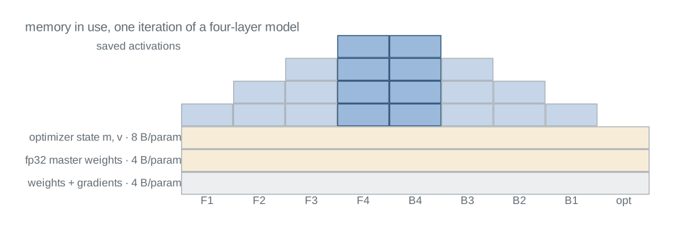
Activation memory sits on top, and unlike the persistent state it scales with . The two are traded against each other constantly: activation checkpointing buys activation memory with compute, while sharding strategies such as ZeRO and FSDP buy persistent memory by partitioning the 16 bytes across workers and gathering them on demand.
5. Compute Accounting
For a dense Transformer with parameters trained on tokens, the standard estimate of total training arithmetic is
where the factor 6 is two FLOPs per parameter for the forward multiply-accumulate and four for the backward pass. With full activation checkpointing the factor rises to about 8. The estimate counts matrix-multiplication work only and ignores attention’s term, so it degrades at very long context.
The useful derived metric is model FLOPs utilization (MFU): achieved divided by the hardware’s peak throughput. MFU normalizes away model size and cluster size, so it is the one number that compares a small run against a large one. Well-tuned large-scale training reaches roughly 40–55% MFU; a run below 25% has a specific, findable problem, and the diagnostic tools in the distributed training article exist to find it.
For choosing and under a fixed budget , the Chinchilla scaling analysis found the compute-optimal allocation scales both roughly equally, giving about 20 tokens per parameter. Models intended for heavy serving are deliberately trained past that point, accepting worse training efficiency for a smaller model that is cheaper at inference.
6. Numerical Precision
Training in pure fp32 wastes both bandwidth and tensor-core throughput. Mixed precision keeps a low-precision copy for the heavy matrix multiplications and an fp32 master copy for the update.
| Format | Exponent / mantissa bits | Behavior in training |
|---|---|---|
| fp32 | 8 / 23 | Baseline; master weights and optimizer state |
| fp16 | 5 / 10 | More mantissa, narrow range; gradients underflow without loss scaling |
| bf16 | 8 / 7 | Same range as fp32, less precision; no loss scaling needed |
fp16’s limited exponent range causes small gradients to flush to zero. Loss scaling fixes this by multiplying the loss by a large factor before the backward pass, shifting the whole gradient distribution into fp16’s representable range, then dividing it out before the update; a dynamic scaler raises the factor when steps succeed and halves it when it detects an overflow. bf16 keeps fp32’s exponent range and needs none of this machinery, which is why it is the default on hardware that supports it.
The fp32 master weights are not redundant. The update is frequently much smaller than the weight it modifies, and in bf16’s 8-bit mantissa such an update rounds to no change at all. Accumulating into fp32 preserves it.
7. The Reference Loop
The whole article, in code:
model = model.to(device)                                   # bf16 autocast below
opt = torch.optim.AdamW(model.parameters(), lr=3e-4,
                        betas=(0.9, 0.95), weight_decay=0.1)
sched = torch.optim.lr_scheduler.OneCycleLR(opt, max_lr=3e-4,
                                            total_steps=max_steps)

for step, batches in enumerate(accumulated(loader, A_accum)):   # 1. data
    for i, (tokens, labels) in enumerate(batches):
        tokens = tokens.to(device, non_blocking=True)
        labels = labels.to(device, non_blocking=True)

        last = (i == A_accum - 1)
        with contextlib.nullcontext() if last else model.no_sync():
            with torch.autocast("cuda", dtype=torch.bfloat16):
                logits = model(tokens)                          # 2. forward
                loss = F.cross_entropy(                         # 3. loss
                    logits[:, :-1].flatten(0, 1),               #    the shift
                    labels[:, 1:].flatten(),
                    ignore_index=-100,                          #    the mask
                ) / A_accum
            loss.backward()                                     # 4. backward
                                                                # 5. sync: in
                                                                #    backward's
                                                                #    hooks
    torch.nn.utils.clip_grad_norm_(model.parameters(), 1.0)     # 6. optimizer
    opt.step()
    sched.step()
    opt.zero_grad(set_to_none=True)
Step 5 has no line of its own, and that is the point. Under DistributedDataParallel, gradient synchronization is triggered from autograd hooks that fire during loss.backward(), so the communication overlaps the computation instead of following it. Understanding that mechanism — and knowing when it fails to overlap — is the subject of part 3.
8. Where the Time Goes
Four things consume wall-clock time in the loop, and they fail in recognizable ways.
| Bucket | What it is | Symptom when dominant |
|---|---|---|
| Data | Reading, decoding, collating, host-to-device copy | GPU idle in a gap before each step; step time tracks worker count, not model size |
| Compute | Forward and backward kernels | Kernels back to back with no gaps; step time scales with , , and |
| Communication | Gradient all-reduce, parameter gathers | Step time flat in but scaling with world size; collective kernels visible and exposed on the timeline |
| Overhead | Python, kernel launches, optimizer, synchronization points | Many short kernels with launch gaps; CPU-side time exceeds GPU time |
The single most common mistake is diagnosing this from nvidia-smi. Its utilization figure reports the fraction of time at least one kernel was resident — not how much of the GPU that kernel used. A training loop stalled on its dataloader and one saturating tensor-core kernel can both read 100%. Distinguishing the four buckets requires a timeline, which means the PyTorch Profiler or Nsight Systems.
9. What This Series Covers Next
Each remaining article takes one part of this loop apart on real hardware.
Tiling and Collective Operations. Arithmetic intensity and the ridge point, how tile size follows from on-chip capacity, why tiles are nested one per level of the memory hierarchy, and the six collective operations of distributed training — broadcast, reduce, all-reduce, reduce-scatter, all-gather, all-to-all — with worked examples and cost models.
PyTorch Distributed Training Internals.
DataParallelversusDistributedDataParallelarchitecture, what NCCL adds to the all-reduce of §3.5, gradient bucketing and the overlap of communication with the backward pass, diagnosing dataloader stalls against compute bottlenecks, and using the PyTorch Profiler and Nsight Systems to tell the buckets of §8 apart.Activations, Normalization and Optimizers, in Plain Terms. What ReLU, GELU, SiLU and SwiGLU each compute and why each replaced the last, LayerNorm against RMSNorm and why placement matters more than the choice, and the one-idea-at-a-time road from SGD through momentum and Adam to AdamW.
Neural Network Quantization. Post-training quantization versus quantization-aware training, per-tensor against per-channel scaling, why attention and normalization layers are disproportionately sensitive to INT8, and the techniques that recover the lost accuracy.
References
- Ashish Vaswani et al. Attention Is All You Need. NeurIPS 2017.
- Ilya Loshchilov and Frank Hutter. Decoupled Weight Decay Regularization. ICLR 2019.
- Paulius Micikevicius et al. Mixed Precision Training. ICLR 2018.
- Tianqi Chen, Bing Xu, Chiyuan Zhang, and Carlos Guestrin. Training Deep Nets with Sublinear Memory Cost. 2016.
- Jared Kaplan et al. Scaling Laws for Neural Language Models. 2020.
- Jordan Hoffmann et al. Training Compute-Optimal Large Language Models. NeurIPS 2022.
- Samyam Rajbhandari, Jeff Rasley, Olatunji Ruwase, and Yuxiong He. ZeRO: Memory Optimizations Toward Training Trillion Parameter Models. SC 2020.
- Deepak Narayanan et al. Efficient Large-Scale Language Model Training on GPU Clusters Using Megatron-LM. SC 2021.