LLM Inference Introduction: the end-to-end flow and vector math

Large Language Models (LLMs) are (mostly) autoregressive models: they predict the next token given the tokens so far, and repeat this loop until stopping. This post focuses on inference: the overall flow, what vectors get computed, and how the attention mechanism combines information across tokens. We also focus on the what data is generated in each phase of an LLC and how they are used in other phases of an inference process.

2. Inference: the end-to-end loop

At a high level, inference is:

1. Tokenize the prompt into token IDs.
2. Embed token IDs into vectors (plus positional information).
3. Run $N_{\mathrm{layers}}$ Transformer blocks (attention + MLP).
4. Produce logits for the next token; convert to probabilities.
5. Select the next token (argmax or sampling), append it, and repeat.

The loop runs until an end condition: max tokens, an EOS token, or a stopping rule.

2.1 Overview

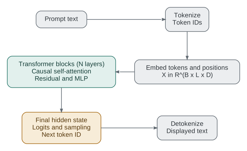
3. Tokenize and Positions embedding

Here, there are $L$ tokens in each prompt, each embedded in a $D$-dimensional space. A batch contains $B$ such prompts.

3.1 Tokenization (text → IDs)

Modern LLMs typically use a subword tokenizer (BPE, Unigram, WordPiece, etc.). The prompt becomes a sequence of token IDs:

where $\|V\|$ is vocabulary size.

Practical notes:

• Tokenization defines the model’s “alphabet.” It impacts context length, efficiency, and what counts as a single step of generation.
• Special tokens (BOS/EOS, system delimiters, etc.) are often inserted by the serving stack.

3.2 Turning token IDs into vectors

3.3 Embedding lookup

The model stores an embedding table $E \in \mathbb{R}^{\|V\| \times D}$.

For each token ID $t_i$, we take a row of this table:

Stacking all tokens gives:

3.4 Positional information

Transformers need position information because attention alone is permutation-invariant. Common approaches:

• Absolute positional embeddings: $X \leftarrow X + P$ with $P \in \mathbb{R}^{B \times L \times D}$.
• Rotary / relative position methods (e.g., RoPE): position is injected into the attention computation (often into $Q$ and $K$) rather than added to $X$.

Either way, the result is an initial tensor $X_0 \in \mathbb{R}^{B \times L \times D}$.

4. Inside one Transformer block (MHA + FFN)

A transformer block is the key block for the success of LLMs. At a high-level, it mixes information across tokens (via attention) and then applies a nonlinear transformation to each token vector (via the MLP/FFN). The mixing step allows the model to build up contextual understanding, due to the presence of positional encoding. While the MLP step allows it to create new features and representations that are not just linear combinations of the input.

4.1 What a Transformer block computes (vectors everywhere)

Each block maps $X_\ell \mapsto X_{\ell+1}$ using (i) multi-head self-attention and (ii) an MLP, typically with residual connections and layer normalization. Here, $\ell \in \{1, \ldots, N_{\mathrm{layers}}\}$ indexes the block number, and $X_\ell \in \mathbb{R}^{B \times L \times D}$ is the hidden-state tensor at that layer.

The exact ordering varies (pre-norm vs post-norm), but the core computations are consistent.

4.2 Complete prefill chain: from $X$ to context-mixed vectors

Let:

• $B$: batch size
• $L$: prompt sequence length
• $D$: model hidden dimension
• $H$: number of attention heads
• $d_h = D / H$: dimension per head
• $D_{\mathrm{ff}}$: FFN intermediate dimension
• $\operatorname{LN}$: layer normalization

Step 1. Input hidden states. The block receives one $D$-dimensional vector for every token position.

Step 2. Pre-attention normalization. Normalize each token vector before forming its attention projections.

Step 3. Query, key, and value projections. Learned linear maps create three views of each normalized token.

Step 4. Split into attention heads. Reshape each projection into $H$ independent $d_h$-dimensional subspaces.

Step 5. Causal attention. Each head scores only current and earlier positions, then forms a weighted sum of values.

Step 6. Merge the heads. Concatenate the per-head results and project them back to the model dimension.

Step 7. Attention residual. Add the attention update to the original, unnormalized block input.

Step 8. Pre-FFN normalization. Normalize the residual state before the position-wise feed-forward network.

Step 9. Feed-forward update. Transform each normalized token independently, then add that update to the residual state.

This is a pre-norm block: layer normalization occurs before attention and before the FFN. Some architectures use a different normalization placement or RMSNorm instead.

Why multiple heads? A single attention head can only learn one “type” of relationship between positions (e.g., syntactic adjacency). With $H$ heads, the model can attend to different aspects simultaneously — one head might track subject–verb agreement, another might focus on nearby tokens, yet another on coreference.

Multi-head attention repeats the attention computation for every head in every transformer layer. For example, Llama 2 7B has 32 layers with 32 attention heads per layer: at each layer, those 32 heads run in parallel on the same token sequence. Conceptually, head $h$ has its own learned $W_Q^{(h)}$, $W_K^{(h)}$, and $W_V^{(h)}$, so it forms different queries, keys, values, and attention weights from the same input.

During decoding, each head also produces its own key and value history. The layer’s KV cache keeps these separately along its head dimension: $K_{\mathrm{cache}}, V_{\mathrm{cache}} \in \mathbb{R}^{B \times H \times t \times d_h}$. Thus, the key/value vectors for one head are not shared with another head; the serving system stores the $H$ distinct per-head histories and reads the appropriate one when computing the next token.

4.4 The causal mask: why it matters

In autoregressive generation the model must not peek at future tokens — token $i$ can only attend to positions $1, \dots, i$. The causal mask enforces this by adding $-\infty$ to illegal positions before softmax, which drives those attention weights to zero.

Why is this critical?

• Without the mask, the model could “cheat” during training by reading the token it is supposed to predict, making the learned weights useless.
• At inference the future tokens don’t exist yet, so the mask matches reality — but it must be present during training so the model learns correct causal distributions.

The residual connection then adds the original input back: $X' = X + \text{MHA}(X)$, so information is never lost. The FFN runs next (§4.5).

4.5 MLP: per-token nonlinearity

The feed-forward network (MLP) applies independently to each position:

where $\sigma$ is often GELU or a gated variant (e.g., SwiGLU). This increases representational capacity beyond linear mixing.

4.6 FFN (feed-forward network): the “feature factory”

In many write-ups, the per-token MLP is called the FFN layer. It is conceptually simple but does a lot of the model’s nonlinear work.

Typical shape choices use an expansion factor $D_{\mathrm{ff}} \gg D$ (often $D_{\mathrm{ff}} \approx 4D$):

with $W_1 \in \mathbb{R}^{D \times D_{\mathrm{ff}}}$ and $W_2 \in \mathbb{R}^{D_{\mathrm{ff}} \times D}$.

Key points for inference:

• The FFN is position-wise: it does not mix tokens (no $L \times L$ interaction). It transforms each token vector independently.
• The compute is dominated by dense GEMMs ($B \times L \times D$ by $D \times D_{\mathrm{ff}}$, then $B \times L \times D_{\mathrm{ff}}$ by $D_{\mathrm{ff}} \times D$), which GPUs handle efficiently.
• Gated variants (e.g., SwiGLU) change the exact formula but keep the same idea: expand $D \to D_{\mathrm{ff}}$, apply a nonlinearity/gate, then project back to $D$.

5. From final vectors to the next token

After $N_{\mathrm{layers}}$ blocks, we have $X_{\mathrm{out}} \in \mathbb{R}^{B \times L \times D}$. To predict the next token for one request, we use its last-position vector $x_L \in \mathbb{R}^D$.

Compute logits over the vocabulary:

Many models tie weights so that $W_U \approx E^T$.

Convert logits to probabilities with temperature $T$:

Temperature rescales every logit before softmax. At $T=1$, the model uses its original distribution; $T<1$ sharpens it toward high-probability tokens, making output more predictable, while $T>1$ flattens it and makes lower-probability tokens more likely. It is useful when the application needs to trade deterministic behavior for variety without changing the model’s weights.

Then choose the next token:

• Greedy decoding: choose $\arg\max_v p(v)$. This is deterministic and useful for reproducible outputs, but can sound repetitive because it always chooses the locally most likely token.
• Top-$k$ sampling: retain only the $k$ most likely tokens, renormalize their probabilities, and sample from that set. This removes an arbitrarily long tail of implausible tokens.
• Nucleus (top-$p$) sampling: retain the smallest set of tokens whose cumulative probability is at least $p$, then renormalize and sample. Unlike top-$k$, the candidate-set size adapts: it grows when the model is uncertain and shrinks when it is confident.
• Repetition penalties: lower the score of tokens that have already appeared in the generated context before sampling. They help prevent loops and copied phrases, but an overly strong penalty can make necessary names or technical terms less likely.

Generation also needs stopping controls: a maximum-token limit bounds runtime and output size; an EOS token lets the model signal completion; and a serving application can define stop sequences such as a chat delimiter to stop at a protocol boundary.

This yields a new token ID $t_{L+1}$, appended to the context, and the loop repeats.

6. Worked example: prefill and two-token decoding

This deliberately small model has one attention head with $D=d_h=2$ and identity projections, so $Q=K=V=X$. It generates two tokens after the prompt I like: first tea, then ..

Use these token vectors:

For the toy output projection, use the following vocabulary vectors:

6.1 Prefill: process the prompt at once

Prefill runs the full prompt through the model in parallel. For I like, the input is:

The causal mask prevents I from seeing like, while like can see both positions. With $Q=K=V=X_{\mathrm{prompt}}$, the masked attention scores and probabilities are:

The final prompt position produces:

At the same time, prefill stores the prompt keys and values for this layer:

Use $h_{like}$ to score the next token:

After softmax, tea has the highest probability, so it is the first generated token. Notice that the first generated token is selected from the last prefill output; it does not require reprocessing the prompt.

6.2 Decode: append tea and generate the second token

The next decode step processes only the newly generated token tea. Its query, key, and value are $q_3=k_3=v_3=[1,1]$. The query attends over the two cached prompt keys plus its new key:

The new hidden state is the weighted value sum:

Append the new key and value rather than recomputing the prompt’s entries:

Now the same output projection selects the second generated token:

The period has the highest probability, so the completed generated suffix is tea .. In a real system, the period would be passed to another one-token decode step unless an EOS token or stop sequence ends generation.

7. What changes during real inference

Real deployments add a few important engineering layers:

• KV cache: during autoregressive decoding, you don’t recompute $K$ and $V$ for all past tokens each step. You cache them per layer and only compute the new token’s projections. What that cache costs, and the attention variants built to shrink it, is the subject of the next article.
• Batching: serving stacks batch multiple requests/tokens to use GPU efficiently.
• Precision: inference often uses FP16/BF16, sometimes INT8/FP8 quantization.
• Decoding policy: sampling settings (temperature, top-$p$, repetition penalties) strongly affect outputs without changing model weights.

8. KV caching: decoding as append-only attention

The key observation is that in autoregressive decoding, at step $t$ you only need one new query (for the new position) but you need keys/values for all positions so far.

For each layer $\ell$, maintain cached matrices:

When a new token arrives, you compute only its projections and append:

Then compute the new query $q_t = x_t W_Q$ and attend over the cached keys/values:

Here $M_t$ is the (trivial) causal mask for this single query row; in practice you just ensure the new token cannot attend to “future” positions (which do not exist yet).

8.1 ASCII timeline

Prefill (prompt length = L): compute all layers on all tokens

tokens:   [ 1   2   3  ...  L ]
cache K:  [k1  k2  k3  ...  kL]
cache V:  [v1  v2  v3  ...  vL]

Decode step L+1 (generate one token): compute only the new token’s q,k,v

new token:                  [ L+1 ]
append K:   [k1  k2  ...  kL | k(L+1)]
append V:   [v1  v2  ...  vL | v(L+1)]

attention for the new token:
q(L+1)  x  [k1..k(L+1)]^T  -> weights over positions 1..L+1  -> weighted sum of [v1..v(L+1)]

8.2 Why it matters

• Compute: without caching, each new token would re-run attention over all previous tokens and recompute their $K,V$ repeatedly. With KV caching, you reuse $K,V$ and only do the “new query against all cached keys” work.
• Asymptotics: prompt processing (“prefill”) is still quadratic in prompt length due to full self-attention, but token-by-token decoding avoids recomputing past projections and is much closer to linear-in-context per generated token.
• Memory: caching costs memory proportional to context length, number of layers, and number of heads (this is often the main throughput limiter at long context).

9. What’s next

Now that you know what each inference step computes, see Intel TPP for LLM Inference for a deep dive into how these operations are accelerated on Intel CPUs — fused GEMM kernels, blocked weight layouts, flash attention with BRGEMM, and OpenMP parallelism.