Introduction
Autoregressive decoding avoids recomputing the past by keeping earlier tokens’ keys and values in a KV cache. The optimizations in this article can be organized around one storage formula:
- : how many token positions are stored. Count positions across all requests, counting a physically shared prefix only once.
- : how many distinct layer states are stored per position. Normally this is the number of layers.
- : how many elements represent each position in each cached layer state. This is where head sharing and latent compression act.
- : how many bytes store each element. This is where KV quantization acts.
This is a payload model for uniform cached records, not a count of padding, allocator waste, quantization metadata, or workspace. With unequal layer formats or retention policies, sum the corresponding payloads instead of using one product.
We will map each optimization to a factor, then separate storage savings from speed: the measured head-sharing sweep reduces bytes eightfold but latency by only about 2.4×. The detailed sections explain the mechanisms behind that difference. This article assumes the decoding loop from LLM Inference Introduction.
1. Why the Cache Exists
Decoding generates one token at a time. Producing token requires attention over all previous positions, which needs their keys and values, and those depend only on tokens already fixed, so they never change once computed.
The cache therefore avoids recomputing past attention, trading a linear amount of storage for quadratic rather than cubic total attention work.
That is the trade the rest of this article is about: the storage is not small.
2. Sizing the Cache
First recover the familiar formula from the four factors. For independent sequences of length , . Without cross-layer sharing, . Ordinary attention stores a key and a value for every KV head, so , where is the KV-head count and the head dimension. Thus one sequence costs
For a fixed architecture and storage precision, the useful form is bytes per token:
and total cost is that constant times the number of live tokens, summed over every sequence in the batch.
The optimization map. Each row changes part of the same product:
| Optimization | Factor | What changes |
|---|---|---|
| Multi-head attention (MHA) | Baseline: , with one KV head per query head. | |
| Grouped-query attention (GQA) | Share KV heads: . | |
| Multi-query attention (MQA) | Share one KV head across all queries: . | |
| Multi-head latent attention (MLA) | Change the cached representation; the DeepSeek-V2 format below uses . | |
| KV quantization | Use fewer bits per element, allowing for scales and other metadata. | |
| Sliding windows or eviction | Retain fewer token positions, with model and quality constraints. | |
| Cross-layer KV sharing | Store fewer distinct layer states where the architecture supports sharing. | |
| Prefix sharing | Store an identical prefix once for multiple requests. |
Paging acts around the product: it reduces allocation waste rather than shrinking each token’s record. Prefix sharing can additionally reduce the stored payload. These are different benefits.
Worked examples. In BF16 ():
| Model | Bytes/token | 8K context | ×32 sequences | ||
|---|---|---|---|---|---|
| 7B, multi-head | 32 | 512 KB | 4.3 GB | 137 GB | |
| 70B, multi-head (hypothetical) | 80 | 2.5 MB | 21.5 GB | 687 GB | |
| 70B, grouped-query (8 groups) | 80 | 320 KB | 2.7 GB | 86 GB |
The middle row is the reason grouped-query attention exists. A 70B model in BF16 has 140 GB of weights, which already needs two 80 GB GPUs; with multi-head attention, one 8K-token sequence would add 21.5 GB, and a batch of 32 would need 687 GB of cache, nearly five times the weights. The bottom row is the same model as actually shipped: the cache falls to an eighth, so that batch of 32 needs 86 GB, which one additional GPU covers.
Three properties of the formula are worth stating plainly.
It is linear in context length. Doubling the context doubles the cache. There is no reuse to exploit; every position must be retained.
It is linear in batch size, with no sharing. Two sequences share weights but never share cache, except for a common prefix, which is exactly the case PagedAttention makes exploitable.
It does not depend on the number of query heads. Only appears. That is the loophole the next section exploits.
The 512 KB figure in the first row is not just arithmetic. Allocating one layer’s cache for one token as a (2, 1, 32, 128) BF16 tensor gives 16,384 bytes, and multiplying by 32 layers gives 524,288 bytes, exactly 512 KB. Every capacity number later in this series is built from that constant, so it is worth confirming once that the formula and the tensor layout agree.
3. Why Decode Is Memory-Bound
The product explains capacity, not latency. For dense decode, reading the retained history often dominates attention time. The memory-transfer component is approximately
A smaller stored payload need not reduce actual traffic or execution time by the same factor. Reuse, tile reloads, dequantization, latent-attention computation, and kernel scheduling all matter. A shared prefix is stored once but can still be read for multiple requests; batching can improve achieved bandwidth without shrinking any record.
Consider one layer of one decode step. Attention over cached positions performs multiply-accumulates for the scores and the same again for the value-weighted sum, so
Their ratio is the arithmetic intensity of attention at decode time:
The context length cancels. What survives is the ratio of query heads to KV heads, the group size, divided by the element width. In BF16 with multi-head attention, where , the intensity is exactly 1 FLOP per byte, against a ridge point of roughly 295 on an H100 (2,000 TFLOP/s BF16 over 3.35 TB/s HBM). Attention at decode time runs at about a three-hundredth of the machine’s arithmetic capability, and no amount of kernel tuning changes that; the operator is reading memory, not computing. The ratio is hardware-independent; only the ridge point it is compared against changes from one GPU to the next.
3.1 Why prefill does more work per byte
The attention math is the same: compute , apply softmax, and multiply by . What changes is the number of query positions processed together within one sequence, not simply the number of requests in a batch. Decode processes one new query; prefill processes many.
For a four-token prompt, causal prefill computes query-key pairs. A decode step processing only the fourth position computes four. Both use the same four positions’ keys and values, but prefill uses the earlier positions repeatedly for different queries. A tiled kernel can load a KV tile into on-chip memory and reuse it across several query rows before discarding it, doing more arithmetic per byte fetched from HBM.
Batching independent decode requests does not provide the same KV reuse, because each request has its own cache; short prefill workloads may also remain limited by launch overhead or insufficient parallelism.
3.2 Measured intensity and the effect of batching
The decode ratio is measurable rather than merely derivable. On a B300 (2,250 TFLOP/s BF16, 8 TB/s HBM, so a ridge point of 281 FLOP/byte), a paged decode kernel with and computes at an arithmetic intensity of 1.0 FLOP/byte at every batch size and context length tested, and reaches at most 75% of HBM peak, while prefill at the same head dimension reaches 78% of compute peak.
| Operation | Shape | TFLOP/s | GB/s | FLOP/byte | % of peak |
|---|---|---|---|---|---|
| prefill | L=16,384 | 1,753 | 428 | 4,096 | 77.9% (compute) |
| decode | B=1, kv=4,096 | 0.5 | 464 | 1.0 | 5.8% |
| decode | B=32, kv=4,096 | 5.4 | 5,400 | 1.0 | 67.5% |
| decode | B=32, kv=16,384 | 6.0 | 6,013 | 1.0 | 75.2% |
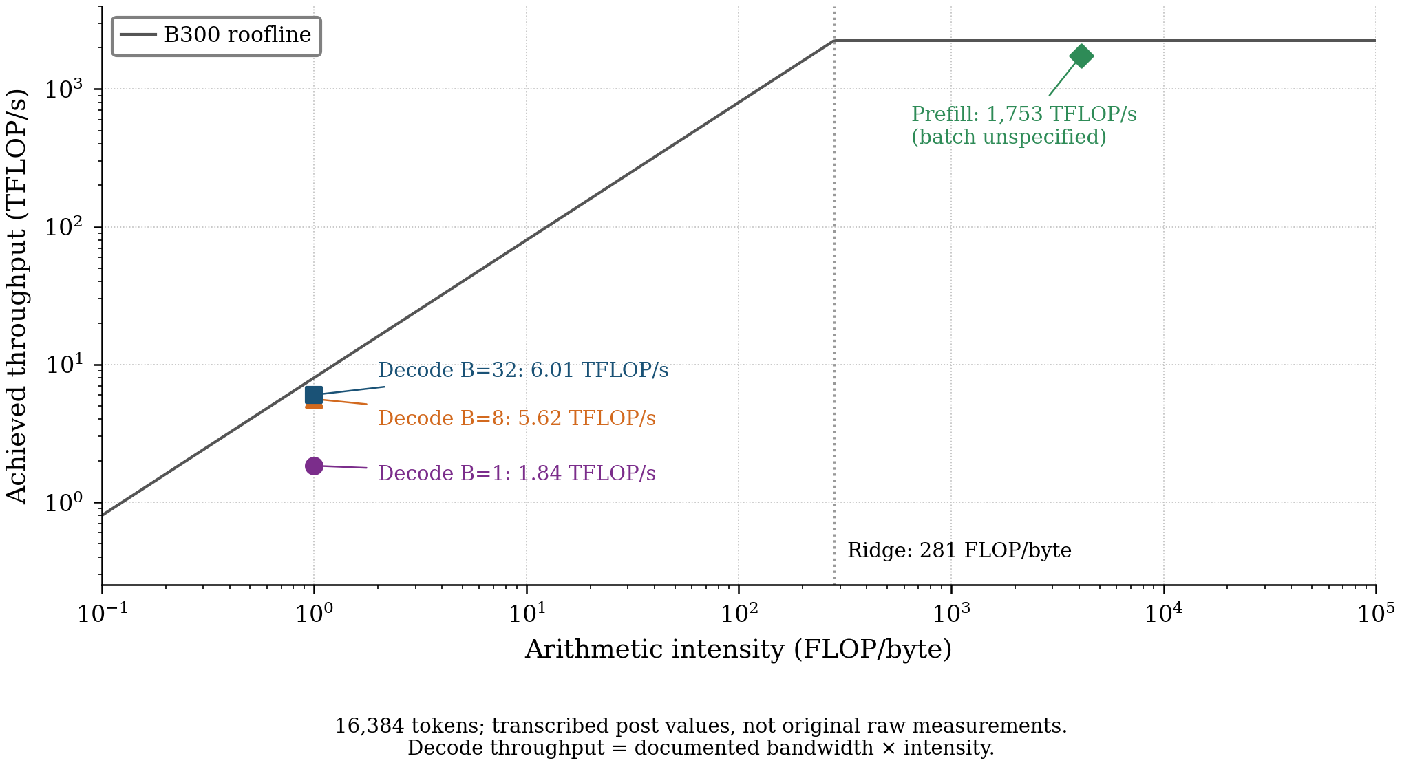
The figure data and plotting script are stored beside the image. From the repository root, run python content/posts/llm-inference-intro/figs/kv-cache-and-attention-variants/plot_roofline.py to regenerate it using the shared acm_style.py helpers.
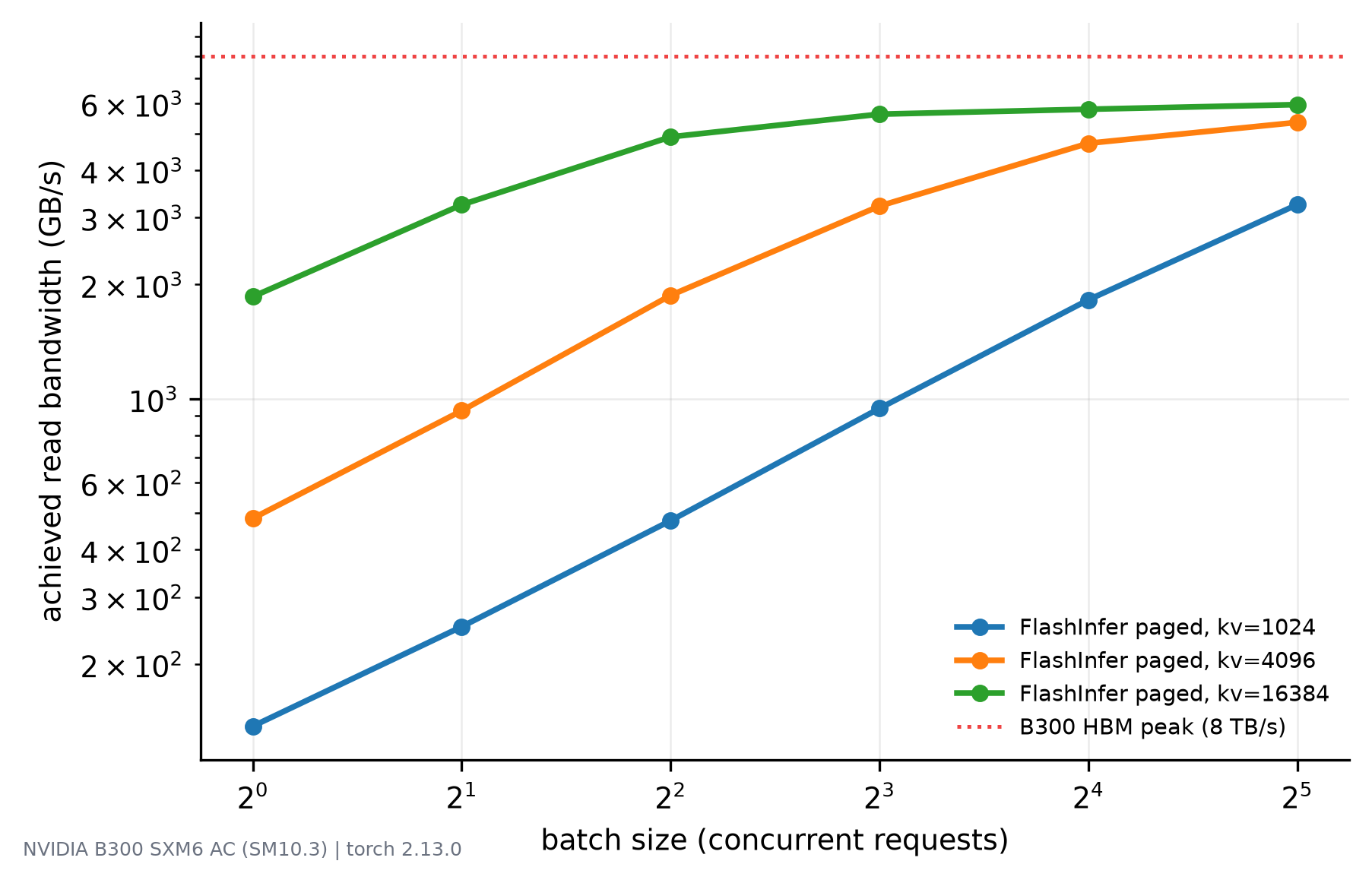
What batching does change is whether the memory system is actually saturated. Those are different statements, and the distinction matters. Measured on the same kernel, at a context length of 16,384:
| Batch | Arithmetic intensity (FLOP/byte) | Achieved read bandwidth | % of HBM peak | Per-request cost |
|---|---|---|---|---|
| 1 | 1.0 | 1,838 GB/s | 23% | 583 µs |
| 8 | 1.0 | 5,621 GB/s | 70% | 77 µs |
| 32 | 1.0 | 6,013 GB/s | 75% | 11 µs |
Intensity never leaves 1.0 FLOP/byte, yet throughput improves 51× per request. The intensity fixes the ceiling, you can never escape the memory roof, while the batch size decides how close to that ceiling you get. A single sequence leaves the HBM channels mostly idle; thirty-two concurrent sequences keep them busy. This is why serving throughput is a scheduling problem, not just a kernel problem.
4. The axis: MHA, MQA, GQA
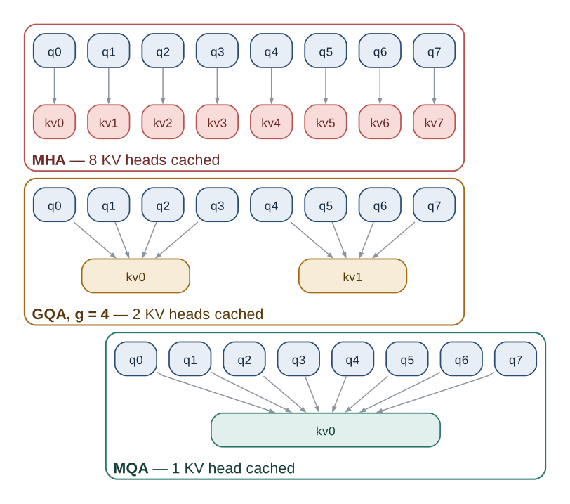
Which factor changes? , the elements stored per token per layer. Hold token count, layer count, head dimension, and precision fixed. MHA, GQA, and MQA retain explicit keys and values but change how many KV heads share the query workload:
All three use the same storage product. MLA also changes , but replaces the explicit KV-head representation rather than choosing another point on this head-sharing axis.
4.1 Multi-head attention (MHA)
Every query head gets its own key and value. Eight query heads, eight KV heads, eight caches per token:
  q0   q1   q2   q3   q4   q5   q6   q7      query heads (H_q = 8)
   |    |    |    |    |    |    |    |
  k0   k1   k2   k3   k4   k5   k6   k7      KV heads  (H_kv = 8)
   |    |    |    |    |    |    |    |
  c0   c1   c2   c3   c4   c5   c6   c7      stored per token

  group size g = 1        KV heads stored = 8        intensity = 2/b
The original: , every head with its own projection. Maximum expressiveness, maximum cache. For the 70B model above it is 2.5 MB per token, which is unaffordable at any serious batch size or context length.
4.2 Multi-query attention (MQA)
Keep all eight query heads, share a single key and value among them:
  q0   q1   q2   q3   q4   q5   q6   q7      query heads (H_q = 8)
   |    |    |    |    |    |    |    |
   +----+----+----+----+----+----+----+---->
                        |
                       k0                    KV heads  (H_kv = 1)
                        |
                       c0                    stored per token

  group size g = 8        KV heads stored = 1        intensity = 16/b
Proposed in 2019 for exactly this reason: keep all query heads but project a single shared key and value. The cache falls by a factor of , 64× for the model above, and decode intensity rises by the same factor.
The cost is quality. Collapsing to one KV head is a real reduction in what attention can represent, and models trained this way show measurable degradation and, in some reports, training instability. MQA is the right answer when memory is the binding constraint and the quality loss is acceptable.
4.3 Grouped-query attention (GQA)
The interpolation, and now the default. Partition the query heads into groups; every head within a group shares one key-value pair. With two groups:
  q0   q1   q2   q3   q4   q5   q6   q7      query heads (H_q = 8)
   |    |    |    |    |    |    |    |
   +----+----+    |    |    +----+----+
        |         |    |         |
       k0         |    |        k1           KV heads  (H_kv = 2)
        |         |    |         |
       c0                     c1             stored per token

  group size g = 4        KV heads stored = 2        intensity = 8/b

  g = 1  <-----------------+-----------------> g = H_q
     MHA                  GQA                   MQA
                        (g = 8 typical)
At , the cache is one eighth of MHA and the intensity is eight times better, with quality close to MHA.
Two practical properties explain its adoption. First, the natural choice is equal to the tensor-parallel degree, so each GPU holds exactly one KV head and no cache is replicated across devices. Second, an existing MHA checkpoint can be converted rather than retrained: mean-pool the key and value projections within each group and continue training for a small fraction of the original budget. Llama 2’s 70B model, Mistral, and most models released since use GQA.
4.4 The variants side by side
| Variant | Cached per token per layer | Relative cache | Decode intensity | Choose when |
|---|---|---|---|---|
| MHA | contexts are short and quality dominates | |||
| GQA, group size | balance quality, cache size, and tensor-parallel layout | |||
| MQA | memory is the binding constraint and you can retrain |
MLA is deliberately absent from that table; it is not on this axis and gets its own section next.
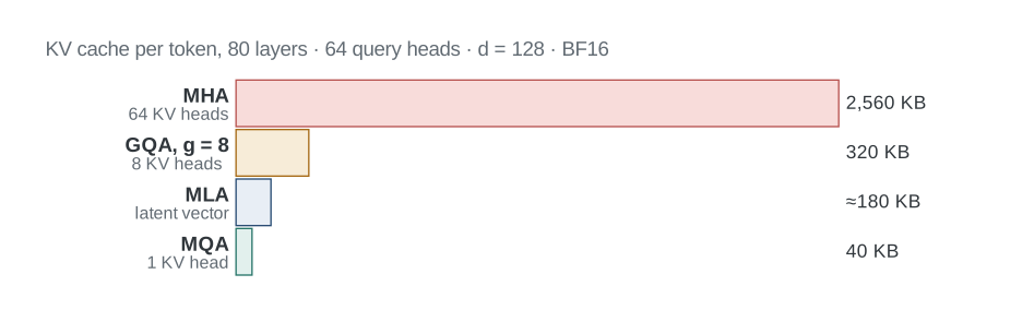
The formulas are worth applying to one concrete model rather than three separate ones. The 70B shape from §2 (, , , BF16) at 8K context:
| Variant | Cache/token | One 8K sequence | ×32 sequences | Intensity | |
|---|---|---|---|---|---|
| MHA | 64 | 2.5 MB | 21.5 GB | 687 GB | 1.0 |
| GQA, | 8 | 320 KB | 2.7 GB | 86 GB | 8.0 |
| MQA | 1 | 40 KB | 335 MB | 10.7 GB | 64.0 |
Going from MHA to GQA divides by eight and makes the payload eight times smaller. The last column describes a different quantity: arithmetic intensity rises eightfold because the query workload remains while fewer KV bytes are read. This creates an opportunity for lower latency, not a guarantee of proportional speedup.
But only up to a point, and the limit is worth stating here rather than leaving to the measurement section: an eight-times reduction in bytes does not buy an eight-times reduction in latency. Measured, it buys about 2.4×.
4.5 What the variants do to the weights
Everything so far has been about the cache. The variants also change the model’s parameter shapes, and they do so asymmetrically, which is the part that is easy to get wrong. Only the key and value projections shrink. The query and output projections keep their full width in every variant.
With the model width:
| Projection | MHA | GQA, group size | MQA |
|---|---|---|---|
The reason is structural rather than incidental. There are always query heads, so must emit columns, and must consume and return . Only the K and V projections emit one column block per KV head, and there are fewer of those.
It is worth being precise here because the phrasing “each head has its own , , ” invites a wrong mental picture. In code there is one matrix, and the heads are slices of its output:
# MHA: Q, K, V all project to D columns
self.W_Q = nn.Linear(D, D)
self.W_K = nn.Linear(D, D)
Q = self.W_Q(X).view(B, L, H_q, d_h).transpose(1, 2)   # heads = column blocks

# GQA: only K and V get narrower
self.W_K = nn.Linear(D, H_kv * d_h)          # D/g columns worth
K = self.W_K(X).view(B, L, H_kv, d_h).transpose(1, 2)
Splitting one weight into column blocks is exactly equivalent to having separate matrices, because a linear layer’s output columns are independent. It is also why production stacks fuse the three projections into one qkv_proj: one GEMM beats three.
Applied to the 70B shape, the asymmetry shows up as a real parameter difference:
| Variant | shape | Attention params/layer | × 80 layers |
|---|---|---|---|
| MHA (hypothetical) | 268 M | 21.5 B | |
| GQA, (as shipped) | 151 M | 12.1 B | |
| MQA | 136 M | 10.9 B |
GQA saves 9.4 billion parameters against multi-head, roughly 13% of a 70B model. That is a larger effect than it first appears, because attention is being compared against itself; the FFN in the same layer is 704 M parameters, so GQA attention (151 M) is about a fifth of the block.
One last consequence is practical, and it explains why the checkpoint-conversion trick in §4.3 works at all. Moving down this table is a reshape: going from MHA to GQA discards columns within each group and averages what remains, which is exactly the mean-pooling operation used to initialise from an existing checkpoint. Moving up, or going to MQA, is not a reshape (87% of ’s columns have no counterpart), so those models are trained from scratch. Shape compatibility runs one way only.
5. Compressing instead of dropping heads: MLA
Which factor changes? Again , but by changing the record rather than sharing explicit KV heads. GQA stores fewer sets of per-head keys and values. MLA instead caches a compact latent representation from which the attention computation obtains the information it needs. It should not be modeled as keeping fixed and compressing each cached head independently.
In the DeepSeek-V2 format, one token’s cached record contains a joint KV latent of dimension plus a decoupled positional component of dimension [3]. In the shared formula, replace the ordinary record size with
DeepSeek-V2 makes those dimensions concrete: compressed plus decoupled RoPE. That is 576 elements per token per layer, against for an equivalent multi-head layer, about 1.8% of the naive per-layer cache. The paper reports roughly a 93% end-to-end reduction; the two figures measure different baselines, since the end-to-end number compares against a sibling model with its own layer count and head configuration rather than against a like-for-like MHA layer. This calculation establishes storage savings, not a latency ratio.
  stored per token, per layer:

     MHA                     MLA
  +---------+            +---------+
  |   k0    |            |         |
  |   k1    |            |  latent |  d_c = 512   compressed K and V
  |   ...   |   ---->    |         |
  | k_{127} |            +---------+
  |   v0    |            |  rope   |  d_r = 64    cannot be compressed
  |   ...   |            +---------+
  | v_{127} |
  +---------+            576 elements
  32,768 elements

  Explicit per-head K and V are replaced by one compact record.
The query heads still exist, but the cached object is no longer a list of independent KV-head vectors. That is why the group-size formula cannot simply be applied to MLA.
The computation changes too. MLA uses down- and up-projections rather than only narrowing and . DeepSeek-V2 describes absorbing the KV up-projections into the query and output projections for inference, avoiding explicit reconstruction of the full cached K and V [3]. Actual speed depends on that execution path and its kernels. A smaller does not by itself establish either fewer total model parameters or faster decoding.
6. Measuring the Variants
The storage formula predicts exactly how head sharing changes . A proportional latency reduction would additionally require unchanged achieved bandwidth and no other dominant cost. The following sweep tests that extra assumption.
Sweep with fixed, so the group size takes the values a real model would choose: is MHA, is MQA. Same kernel, same page size, same dtype; only the head axis of the cache changes. At a 16K context and batch 32:
| bytes read per step | latency | speedup | achieved GB/s | % of HBM peak | ||
|---|---|---|---|---|---|---|
| 8 (MHA) | 1 | 2048 MB | 0.360 ms | 1.00× | 5,966 | 74.6% |
| 4 | 2 | 1024 MB | 0.214 ms | 1.68× | 5,008 | 62.6% |
| 2 | 4 | 512 MB | 0.177 ms | 2.04× | 3,037 | 38.0% |
| 1 (MQA) | 8 | 256 MB | 0.152 ms | 2.38× | 1,772 | 22.1% |
Bytes fall by exactly the factor the formula predicts: eight. Latency falls by 2.38×. The prediction is wrong by a factor of 3.4, and it is not wrong because the machine was idle. Repeating the sweep at batch 64 and 64K context, where the baseline already sustains 88.9% of peak, still yields only 2.12×.
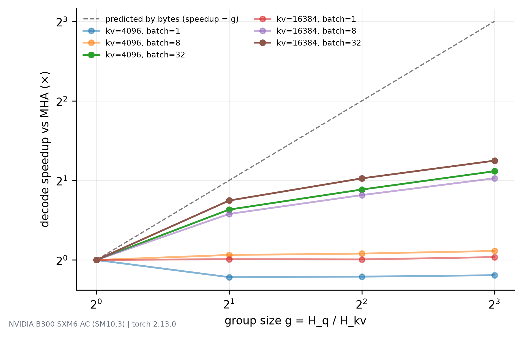
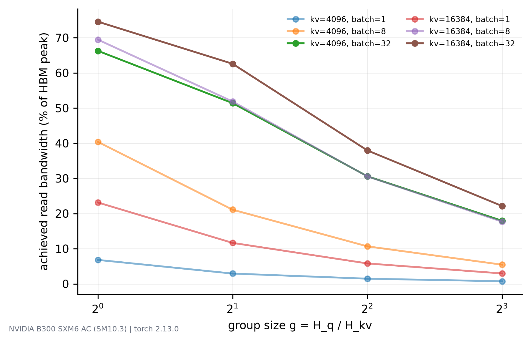
The obvious explanation, that narrower reads coalesce worse, turns out to be wrong, and it is worth showing the falsification rather than asserting the answer. In the standard NHD layout the contiguous run for one token is bytes, so the two candidates are access granularity and parallelism. Both can be varied independently.
Hold the head count at one and widen the contiguous run by raising , and bandwidth does not move at all:
| contiguous run | achieved GB/s | % of peak | |
|---|---|---|---|
| 64 | 128 B | 1,647 | 20.6% |
| 128 | 256 B | 1,779 | 22.2% |
| 256 | 512 B | 1,747 | 21.8% |
| 512 | 1024 B | 1,739 | 21.7% |
An eight-times wider slice changed bandwidth by one percentage point, while latency tracked bytes exactly. Access granularity is not the cause. Nor is parallelism: at fixed , going from 16 to 512 concurrent requests, 32× more independent streams, moved bandwidth only from 19.7% to 24.0%.
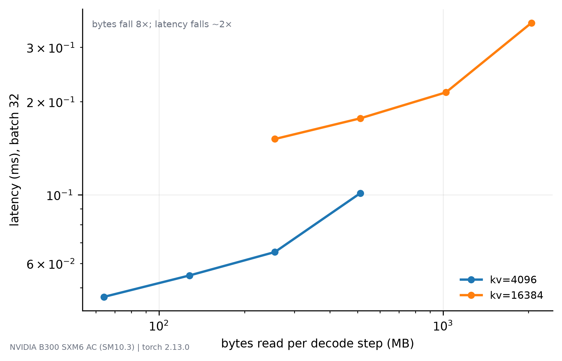
Return to the product: the sweep reduces , but keeps the query-head count and context fixed. The leading score and value arithmetic therefore stays roughly constant while bytes fall; work per byte rises with . Non-memory costs can consequently become more visible. Identifying the specific bottleneck would require instruction-level profiling, not just effective-bandwidth measurements.
Three consequences follow, and they are more useful than the prediction was.
A smaller has diminishing latency returns in this sweep. The last doubling of from 4 to 8 bought 17% of latency while costing more than half the bandwidth efficiency. That is a workload-specific trade-off, not a universal optimum at .
MLA needs its own performance measurement. Its smaller latent record reduces , but also changes the computation. The MHA/GQA sweep cannot predict MLA’s work per byte or guarantee that it avoids the same latency plateau.
Different factors have different runtime consequences. Quantization reduces but adds conversion work; a window reduces and the number of attended positions; sharing cached state saves storage without necessarily removing each consumer’s reads. The product tells us what to count, while measurements establish what gets faster.
7. The Other Levers
Return to . Head sharing and MLA change ; the remaining levers change how many records are kept, how often they are stored, or how their elements are encoded. They can compose where the model and serving engine support them.
Quantize it: reduce . The cache is a tensor like any other. Quantizing it from BF16 to an 8-bit format halves the element payload; a packed 4-bit format quarters it. The 512 KB/token example becomes 256 KB/token or 128 KB/token before scales, zero points, padding, and any higher-precision residuals. The representation size need not change.
This also illustrates composition with MLA: its 576-element record occupies payload bytes in BF16, or 576 bytes in an 8-bit encoding, if supported. These are storage calculations, not measured speedups or quality guarantees. Quantization adds conversion work and can affect quality. KIVI finds that keys benefit from per-channel quantization while values benefit from per-token quantization [7], so metadata and scaling choices matter.
For ordinary MHA, the idealized intensity rises from 1 to 2 FLOP/byte when element width halves. That is more work per byte, not constant work per byte. Whether latency improves proportionally depends on conversion overhead and achieved bandwidth.
Bound what is kept: reduce . For independent requests with a supported window of tokens, rather than . Attention-sink methods retain a small initial prefix alongside recent tokens [6]; eviction policies discard selected positions. These change which history remains available and require model compatibility or quality evaluation, unlike merely storing the same elements at lower precision.
Share across layers: reduce . If an architecture lets each set of layers share one cached state, for equal-size groups. This reduces the number of stored records, not the number of Transformer layers or necessarily the number of reads. It is an architectural feature, not an arbitrary inference-time substitution.
Share prefixes: reduce physical . If requests share an identical reusable prefix of tokens and each has a private continuation of tokens, separate storage needs positions; sharing needs only . Each request still performs its own attention, so storage sharing alone does not guarantee shared reads.
Stop wasting what you allocate: reduce overhead around the product. PagedAttention allocates cache blocks on demand rather than reserving a request’s maximum future length [5]. It reduces over-reservation and fragmentation, though a partly filled final block can still waste space. Prefix sharing is an additional way to reduce the payload itself. Neither mechanism changes or .
8. What This Means for a Serving System
Use the formula as a checklist: which factor changes, what does the engine actually allocate and read, and which runtime cost remains?
The cache sets the batch-size ceiling at long context. Weights are a fixed cost paid once; cache is a per-sequence cost that grows with the context. Past a few thousand tokens the cache is the term that decides how many requests fit, which is why throughput at 32K context looks nothing like throughput at 512.
Payload savings and speedups are separate results. Use to estimate stored bytes, then evaluate actual traffic, achieved bandwidth, computation, and conversion overhead. In §6, reducing eightfold gives about 2.4× lower latency. That result does not predict the speedup from quantizing , changing MLA’s record format, or sharing physical prefixes.
Prefill and decode want different things. Prefill processes many query positions together and can become compute-bound; decode processes one new query per request and often depends on KV-read bandwidth. Batching improves device occupancy and bandwidth use without shrinking each record. It optimizes execution around the storage formula rather than changing the record size.
9. Summary
- Start with : stored token positions, distinct cached layer states, elements per record, and bytes per element.
- MHA, GQA, and MQA change through KV-head sharing. MLA changes by storing a latent record instead of explicit per-head K and V.
- Quantization reduces ; windows and prefix sharing reduce ; cross-layer sharing reduces . Paging reduces allocation overhead around the payload.
- Storage savings are not latency guarantees. In the measured head-sharing sweep, bytes fall eightfold but latency improves about 2.4× as achieved bandwidth drops. MLA and quantization require their own measurements.
- Batching optimizes execution. It can improve bandwidth use at unchanged decode intensity without shrinking the persistent KV record.
References
- Noam Shazeer. Fast Transformer Decoding: One Write-Head is All You Need. 2019.
- Joshua Ainslie et al. GQA: Training Generalized Multi-Query Transformer Models from Multi-Head Checkpoints. EMNLP 2023.
- DeepSeek-AI. DeepSeek-V2: A Strong, Economical, and Efficient Mixture-of-Experts Language Model. 2024.
- Reiner Pope et al. Efficiently Scaling Transformer Inference. MLSys 2023.
- Woosuk Kwon et al. Efficient Memory Management for Large Language Model Serving with PagedAttention. SOSP 2023.
- Guangxuan Xiao et al. Efficient Streaming Language Models with Attention Sinks. ICLR 2024.
- Zirui Liu et al. KIVI: A Tuning-Free Asymmetric 2bit Quantization for KV Cache. ICML 2024.