Everything on Precision: Numeric Formats in Modern ML and HPC
Every number in a computation carries a cost: it occupies memory, travels the bus, and burns ALU cycles when it meets another number. The format you store and compute in — the precision — is one of the most consequential choices in any ML or HPC pipeline. Get it wrong and you either waste half your hardware or silently wreck your model.
This post covers the formats that matter today — FP32, TF32, FP16, BF16, FP8, INT8, INT4 — with emphasis on how they actually behave, when each one is appropriate, and where the pitfalls hide.
1. The Basics: What a Number Format Gives You (and Takes Away)
A numeric format pins down three things:
- Range — how large or small a value can get before it overflows or underflows.
- Resolution — how finely you can distinguish nearby values.
- Cost — how many bytes you move and how many ops-per-cycle your hardware can deliver.
In practice, cost dominates. For large matrix multiplications arithmetic scales as while data movement scales as . Halving the byte-width of your operands roughly halves communication time while barely touching the compute wall. This is why lower-precision paths are often faster even when nominal peak FLOP rates look similar — the savings come from reduced memory traffic, not faster arithmetic.
1.1 A quick scaling example
Consider a square GEMM (General Matrix Multiply): with .
- Compute: ~ FLOPs.
- For each of the output elements, you do multiplies and adds: .
- With fused multiply-accumulate, the multiply count equals the add count, giving exactly FLOPs.
- One-pass data: ~ elements → roughly bytes in FP32.
- You need to read and once, and write once. Each element is 4 bytes in FP32, so total bytes = .
- In a different data type say FP16, the total bytes = .
Table 1: Compute () vs data movement () for a square GEMM.
| N | Compute FLOPs | Data bytes (FP32) |
|---|---|---|
| 256 | 33,554,432 (~33.6 M) | 786,432 (~0.75 MiB) |
| 512 | 268,435,456 (~268.4 M) | 3,145,728 (~3.00 MiB) |
| 1024 | 2,147,483,648 (~2.15 B) | 12,582,912 (~12.0 MiB) |
Double and compute grows while data grows only . At large enough the hardware spends most of its time on arithmetic, not waiting for memory — this is the “compute-bound” regime.
Once there, cutting the data term in half (e.g., FP32 → BF16) barely affects the compute wall but meaningfully reduces load/store traffic. You also tend to fit a larger working set in cache. The throughput win is larger than “half the bits” might suggest.
1.2 How floating-point numbers are stored
A floating-point number is split into three fields:
- Sign (1 bit) — positive or negative.
- Exponent ( bits) — a power of 2 that sets the magnitude; controls range.
- Mantissa ( bits, also called the significand or fraction) — the significant digits; controls precision.
The encoded value is:
The leading 1. is implicit (always present, never stored), giving one extra bit of precision for free. The bias avoids storing negative exponents: with exponent bits, bias = . The real exponent is simply stored_exponent − bias.
Why the bias matters. Numbers smaller than 1.0 need negative exponents, but storing signed integers in the exponent field complicates hardware comparisons. The bias sidesteps this: all exponents are stored as unsigned integers, yet negative real exponents are fully representable:
- 0.375 in FP32: . The real exponent is , but we store (unsigned). No negative number anywhere in the bit pattern.
- 0.001953125 in FP32: . The real exponent is , stored as . Again, a simple unsigned integer.
Without bias these exponents would be and , requiring signed arithmetic for comparisons. With bias, comparing two positive floats reduces to an unsigned integer comparison.
Worked example (FP32-style).
- Sign = 0 (positive), stored exponent =
10000001(decimal 129), mantissa bits =01000000000000000000000 - Real exponent = (bias is 127 for 8-bit exponents).
- The mantissa encodes (remember the implicit leading 1).
- Value: . Flip the sign bit → .
1.3 The exponent-vs-mantissa trade-off: BF16 vs FP16
BF16 and FP16 are both 16 bits, but they spend those bits differently:
| Exponent bits | Mantissa bits | |
|---|---|---|
| BF16 | 8 | 7 |
| FP16 | 5 | 10 |
More exponent bits buy wider range; more mantissa bits buy finer precision.
- BF16 keeps FP32’s 8-bit exponent, so it covers the same dynamic range. Gradients and activations that would overflow FP16 fit comfortably in BF16.
- FP16 trades range for precision. Near 1.0, consecutive representable values are ~ apart (FP16) versus ~ apart (BF16) — about 8× finer.
In short: FP16 gives better precision when values stay in a narrow band; BF16 is more robust when they do not.
1.4 Integer quantization (INT8 / INT4)
Integer formats have no exponent or mantissa — just fixed-width signed values ( to for INT8, to for INT4). To map floating-point tensors into this representation you quantize:
where is a scale factor and is a zero-point (often 0 in symmetric mode).
Example: Suppose you have a tensor with values in and want to quantize to INT8 ( to ) with symmetric mode ():
- Scale: .
- Quantize : .
- Dequantize: . The error is — small, but not zero.
- Quantize : . Dequantize: . The value is completely lost — it was smaller than one quantization step.
Key design choices include per-tensor vs per-channel scales, symmetric vs asymmetric quantization, and static vs dynamic calibration. These paths trade calibration complexity for big gains in throughput and memory.
2. The Formats: Specs, Strengths, and Weaknesses
2.1 All formats at a glance
Table 2: Numeric precision comparison — range and resolution for each format.
| Format | Bits | Exponent | Mantissa | Dynamic Range (approx) | Relative Precision |
|---|---|---|---|---|---|
| FP32 | 32 | 8 | 23 | ~ to ~ | ~1.19e-7 |
| TF32 | 19 eff. | 8 | 10 | ~ to ~ | ~9.77e-4 |
| FP16 | 16 | 5 | 10 | ~ to ~ | ~9.77e-4 |
| BF16 | 16 | 8 | 7 | ~ to ~ | ~7.81e-3 |
| FP8 E4M3 | 8 | 4 | 3 | ~1.56e-2 to ~4.48e2 | coarse |
| FP8 E5M2 | 8 | 5 | 2 | ~ to ~ | very coarse |
| INT8 | 8 | N/A | N/A | −128 to 127 | scale-dependent |
| INT4 | 4 | N/A | N/A | −8 to 7 | scale-dependent |
INT8/INT4 show N/A for exponent and mantissa because they are integer formats — plain fixed-width values, not floating-point encodings.
2.2 FP32
The workhorse for decades. Numerically stable, deterministic, well-tooled — but it costs 2× the memory and bandwidth of 16-bit formats and gets lower throughput on modern tensor/matrix units. Still the right choice for master weights, sensitive reductions, and as a debugging reference.
2.3 TF32 (hardware compute mode, mainly NVIDIA)
From the programmer’s side TF32 looks like FP32, but tensor cores internally truncate the mantissa to 10 bits. This is often free speed for existing FP32 code, though anyone expecting bitwise reproducibility will be surprised. Note that TF32 is a compute mode, not a storage format.
2.4 FP16
Mature accelerator support and good memory savings. The downside is a narrow 5-bit exponent: overflow and underflow are real risks, so training typically requires loss scaling. Works well for inference and mixed-precision training when you have tight scale control.
2.5 BF16
FP32-like range in 16 bits — far fewer overflow headaches than FP16. The coarser mantissa means accumulation strategy matters (accumulate into FP32 whenever possible). BF16 has become the default training dtype on most datacenter hardware, and for good reason.
2.6 FP8 (E4M3 / E5M2)
Still the frontier. Very high throughput and memory efficiency, increasingly viable for both inference and training when paired with careful scaling recipes. E4M3 offers slightly better precision for forward passes; E5M2 has wider range for heavy-tailed distributions. Framework and kernel coverage is still catching up.
2.7 INT8
4× smaller than FP32, 2× smaller than 16-bit formats, with strong ecosystem support across CV, NLP, and recommendation workloads. The cost of entry is calibration and per-layer policy tuning: outlier-heavy layers will degrade quality if not handled carefully.
2.8 INT4
Maximum compression. Excellent cost/performance for LLM serving when paired with good dequantization kernels and group-wise scaling. Quality risk is considerably higher than INT8 — model-specific validation and often outlier routing are required to make it work.
2.9 Summary
Table 3: Quick-reference trade-offs — strengths, weaknesses, and typical usage.
| Format | Main Pros | Main Cons | Typical Role |
|---|---|---|---|
| FP32 | Stable, accurate, easy debugging | Slow, memory-heavy | Reference, sensitive ops |
| TF32 | FP32-range compute, high tensor throughput | Backend-dependent, not a storage dtype | Fast FP32-like training |
| FP16 | Fast, compact | Narrow range, scaling complexity | Mixed training / inference |
| BF16 | Range-friendly, stable mixed training | Coarser mantissa | Training default on many platforms |
| FP8 E4M3 | Better FP8 precision for forward paths | Narrower range than E5M2 | FP8 inference / selected training |
| FP8 E5M2 | Wider FP8 range for hard distributions | Very coarse mantissa | FP8 training paths needing range |
| INT8 | Excellent inference economics | Quantization complexity | Production inference |
| INT4 | Maximum efficiency | Higher quality risk | Cost-optimized inference |
3. Where Errors Come From (and How to Fight Them)
Choosing a format means choosing which errors you can tolerate. Knowing where they enter makes them easier to control.
3.1 Accumulation: the hidden lever
One pattern shows up everywhere in high-performance kernels: multiply in low precision, accumulate in high precision. BF16 × BF16 with FP32 accumulation; INT8 × INT8 with INT32 accumulation. This single design choice — the accumulator width — often matters more for output quality than the input precision.
A dot product is a long chain of multiply-add operations. Each individual product may be fine in low precision, but summing hundreds or thousands of them compounds the rounding errors. A wider accumulator captures the trailing bits that the narrower format would discard at every step.
Example 1: BF16 accumulation vs FP32 accumulation. Consider summing 1000 BF16 values, each equal to . The true answer is .
- BF16 accumulator: BF16’s step size near 1.0 is ~0.0078. Once the running sum reaches ~1.0, adding 0.001 is smaller than the rounding step — so many of the later additions simply vanish. The final sum drifts noticeably below 1.0.
- FP32 accumulator: FP32’s step size near 1.0 is ~ — millions of times finer. Every 0.001 addition is captured accurately. The result is 1.0 (or extremely close to it).
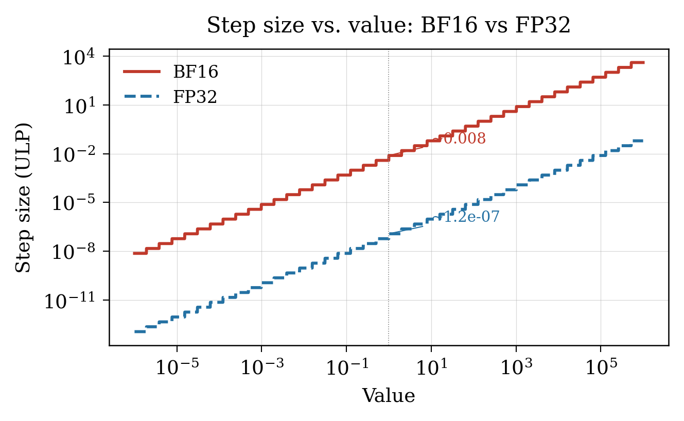
Note that the step size is not constant — it grows with the magnitude of the value. For a format with mantissa bits, the step (also called ULP, unit in the last place) at value is:
identifies which power-of-2 interval falls in (values in give 0, values in give 1, and so on). Within each interval the step is constant at times the interval width, and it doubles when the value crosses the next power of two. Precision is always relative.
Concretely, near 1.0: BF16 () has step ; FP32 () has step . The ratio is ×. The figure below shows this relationship across the full value range:
Same inputs, same multiplications — the accumulator width alone moves the result from “roughly correct” to “essentially exact.”
Example 2: INT8 × INT8 — why INT32 accumulation matters. Take a dot product of two 256-element INT8 vectors. Each product can reach . Summing 256 such products gives a worst-case total of ~4.1 million — well beyond INT16 (max 32767) but easily within INT32 (max ~2.1 billion). Without a 32-bit accumulator the partial sums silently wrap around.
The point is straightforward: inputs can be narrow, but the running total needs headroom. This is why essentially every hardware dot-product unit — NVIDIA tensor cores, Intel AMX tiles, etc. — pairs narrow input operands with a wider accumulator.
3.2 What can go wrong (cons)
Table 4: Common error sources in low-precision computation.
| Error Source | What Happens | Toy Example |
|---|---|---|
| Rounding error | Every multiply/add can silently lose trailing bits, and the errors compound over long reductions. | BF16 step size near 1.0 is ~0.0078, so 1.0 + 0.003 rounds back to 1.0 — the small value just vanishes. |
| Overflow / underflow | Limited exponent range clips extreme values without warning. | FP16 max is 65504. A gradient update that produces 65600 silently becomes inf and poisons the entire backward pass. |
| Quantization bias | A poorly chosen scale/zero-point introduces a systematic shift across all values. | INT8 with scale = 0.1: both 0.03 and 0.07 quantize to q = 1 → both reconstruct as 0.1. Small differences are erased. |
| Outlier clipping | In INT8/INT4, one large activation forces a wide scale, crushing the resolution for everything else. | Tensor range is mostly ±1.0, but one channel hits 100.0. INT8 scale becomes ~0.78, so values near 1.0 all map to q = 1 — you lose almost all information. |
| Sensitive operators | Certain layers amplify small numeric errors far more than others. | Softmax: a rounding error of 0.01 in a logit shifts the output probability by ~1%. Layer-norm: variance computed over thousands of near-equal values is reduction-heavy and drift-prone. |
3.3 How to fight back (pros / mitigations)
Table 5: Practical mitigations and why they work.
| Mitigation | How It Helps | Toy Example |
|---|---|---|
| Higher-precision accumulation | Multiply in low precision but accumulate partial sums in a wider type — catches rounding drift before it snowballs. | BF16 × BF16 → FP32 acc: summing 1000 products stays accurate to ~7 decimal digits instead of ~2. |
| Sensitive-op fallback | Keep numerically critical operators (softmax, layer-norm, optimizer state updates) in FP32/BF16 even when the rest of the model runs in INT8. | Run softmax in FP32: costs <1% extra compute but prevents the exponential from magnifying rounding errors into wrong top-1 predictions. |
| Per-channel / group-wise scales | Finer quantization granularity lets each channel or group use its own scale, reducing clipping and bias. | Per-channel INT8: a channel with range ±2.0 gets scale ≈ 0.016; a channel with range ±50.0 gets scale ≈ 0.39. Neither wastes dynamic range. |
| Outlier routing | Route the small fraction of extreme-value channels to a higher-precision path; quantize the rest aggressively. | 1% of channels have activations >10× the median. Run those in FP16; quantize the remaining 99% to INT8. Quality stays close to FP32 at ~INT8 throughput. |
| Continuous numeric validation | Monitor intermediate tensor distributions (not just final metrics) — catch drift before it becomes a visible accuracy drop. | Log per-layer activation min/max/variance every N training steps. If a layer’s range suddenly doubles, you know precision is under stress before eval metrics move. |
4. Practical Defaults
The typical precision assignments that have emerged from all the trade-offs above:
Table 6: Common precision assignments for training and inference.
| Weights | Activations | Accumulation | |
|---|---|---|---|
| Training | BF16 / FP16 | BF16 (or FP16 + loss scaling) | FP32 |
| Inference | INT8 (INT4 where validated) | INT8 or BF16 | INT32 / FP32 |
Master weights and optimizer states are typically kept in FP32. BF16 is the safer training default since it avoids loss scaling.
Beyond arithmetic, precision choices affect memory capacity (narrower dtypes → larger batches), memory bandwidth (often the real bottleneck), and interconnect cost (all-reduce payloads shrink proportionally). But the best format on paper is useless without an optimized kernel for your target hardware.
Final Thoughts
Precision is a first-order systems decision, not an afterthought. The gains from lower precision come primarily from moving fewer bytes and unlocking specialized hardware paths, not from reducing arithmetic cost. BF16 has earned its place as the training default; INT8 remains the standard for production inference; INT4 and FP8 are increasingly practical but demand careful engineering.
If there is one line to take away: go as narrow as your quality and stability budget allows, and no narrower.
Portions of this post were drafted with the assistance of AI and subsequently reviewed and edited for accuracy.